Bayesian Gravity Inversion: Complete Workflow

This tutorial provides a comprehensive walkthrough of Bayesian gravity inversion using the GemPy-Probability framework. We’ll explore both the theoretical foundations and practical implementation of inferring geological parameters from gravity observations.

What are we doing?

We’re performing Bayesian inference on a geological model using gravity measurements. The goal is to estimate geological parameters such as:

• Dips: Orientation angles of geological layers (degrees)

• Densities: Rock densities for different lithological units (g/cm³)

Why Bayesian Inference?

Bayesian inference provides several advantages over traditional deterministic approaches:

1. Posterior probability distributions: Not just point estimates, but full probability distributions that quantify uncertainty in our parameter estimates.

2. Uncertainty quantification: Explicit characterization of what we know and don’t know about the subsurface.

3. Prior knowledge incorporation: Ability to incorporate geological expertise, physical constraints, and previous studies into the inversion.

4. Outlier detection: Identification of problematic measurements or model misspecification through hierarchical modeling.

The Bayesian Framework

In Bayesian inference, we update our beliefs about parameters θ (e.g., dips, densities) given observed data y (gravity measurements) using Bayes’ theorem:

\[p(θ|y) = \frac{p(y|θ) p(θ)}{p(y)}\]

Where:

• p(θ|y): Posterior distribution - our updated beliefs after seeing the data

• p(y|θ): Likelihood - probability of observing the data given parameters

• p(θ): Prior distribution - our initial beliefs before seeing data

• p(y): Evidence - normalizing constant (marginal likelihood)

The Forward Model

Unlike linear regression where the relationship between parameters and observations is simple (e.g., y = θ₁x + θ₂), here we have a complex forward model:

\[y = f(θ) + ε\]

Where:

• y: Observed gravity at measurement stations

• f(θ): Complex forward model combining geological interpolation and gravity computation

• θ: Parameters (dips, densities, orientations)

• ε: Measurement noise (we’ll model this hierarchically)

The forward model f involves:

1. Geological interpolation (potential field method)

2. Computing density distributions

3. Forward gravity calculation at observation points

4. Normalization and alignment to observations

Import Libraries

import os
import dotenv

dotenv.load_dotenv()

from gempy_probability.modules.plot.plot_posterior import default_red, default_blue
from mineye.GeoModel.model_one.visualization import probability_fields_for
from mineye.GeoModel.model_one.visualization import gempy_viz, plot_many_observed_vs_forward, generate_gravity_uncertainty_plots

from mineye.GeoModel.plotting.probabilistic_analysis import plot_geophysics_comparison

import numpy as np
import matplotlib.pyplot as plt

import gempy as gp
import gempy_probability as gpp
import gempy_viewer as gpv

import torch
import pyro
import pyro.distributions as dist

import arviz as az
from gempy_probability.core.samplers_data import NUTSConfig

# Set random seeds for reproducibility
seed = 4003
pyro.set_rng_seed(seed)
torch.manual_seed(seed)
np.random.seed(1234)

Setting Backend To: AvailableBackends.PYTORCH

Import helper functions

from mineye.config import paths
from mineye.GeoModel.geophysics import align_forward_to_observed
from mineye.GeoModel.model_one.model_setup import baseline, setup_geomodel, read_gravity
from mineye.GeoModel.model_one.probabilistic_model import normalize, set_priors
from mineye.GeoModel.model_one.probabilistic_model_likelihoods import generate_multigravity_likelihood_hierarchical_per_station

Define Model Extent and Resolution

min_x = -707_521
max_x = -675558
min_y = 4526832
max_y = 4551949
max_z = 505
model_depth = -500
extent = [min_x, max_x, min_y, max_y, model_depth, max_z]

# Model resolution: use octree with refinement level 5
resolution = None
refinement = 5

Get Data Paths

mod_or_path = paths.get_orientations_path()
mod_pts_path = paths.get_points_path()
geophysical_dir = paths.get_geophysical_dir()

print(f"Orientations: {mod_or_path}")
print(f"Points: {mod_pts_path}")
print(f"Geophysical data: {geophysical_dir}")

Orientations: /home/leguark/PycharmProjects/Mineye-Terranigma/examples/Data/Model_Input_Data/Simple-Models/orientations_mod.csv
Points: /home/leguark/PycharmProjects/Mineye-Terranigma/examples/Data/Model_Input_Data/Simple-Models/points_mod.csv
Geophysical data: /home/leguark/PycharmProjects/Mineye-Terranigma/examples/Data/General_Input_Data/Geophysical_Cleaned_Data

Create Initial GemPy Model

simple_geo_model = gp.create_geomodel(
    project_name='gravity_inversion',
    extent=extent,
    refinement=refinement,
    resolution=resolution,
    importer_helper=gp.data.ImporterHelper(
        path_to_orientations=mod_or_path,
        path_to_surface_points=mod_pts_path,
    )
)

gp.map_stack_to_surfaces(
    gempy_model=simple_geo_model,
    mapping_object={
            "Tournaisian_Plutonites": ["Tournaisian Plutonites"],
    }
)

Structural Groups:	StructuralGroup: Name: Tournaisian_Plutonites Structural Relation: StackRelationType.ERODE Elements: StructuralElement: Name: Tournaisian Plutonites
Fault Relations:	Tournaisia... Tournaisian_Plutonites
	True False

Step 1: Load Gravity Observations

What is gravity data?

Gravity measurements record variations in Earth’s gravitational field at the surface. These variations arise from lateral density contrasts in the subsurface. Dense rocks (e.g., mafic intrusions) create positive anomalies, while less dense rocks (e.g., sediments) create negative anomalies.

Units: Gravity is measured in microGals (µGal), where 1 µGal = 10⁻⁸ m/s². Typical gravity anomalies from geological structures range from tens to thousands of µGal.

The data includes:

• gravity_data: Station locations (x, y, z coordinates)

• observed_gravity_ugal: Measured gravity values in microGals

gravity_data, observed_gravity_ugal = read_gravity(geophysical_dir)
print(f"\nGravity observations:")
print(f"  Number of measurements: {len(observed_gravity_ugal)}")
print(f"  Range: {observed_gravity_ugal.min():.1f} to {observed_gravity_ugal.max():.1f} µGal")
print(f"  Mean: {observed_gravity_ugal.mean():.1f} µGal")

Gravity observations:
  Number of measurements: 20
  Range: 11717.0 to 39037.0 µGal
  Mean: 25535.6 µGal

Step 2: Setup Geomodel with Gravity Configuration

Geological Model Setup

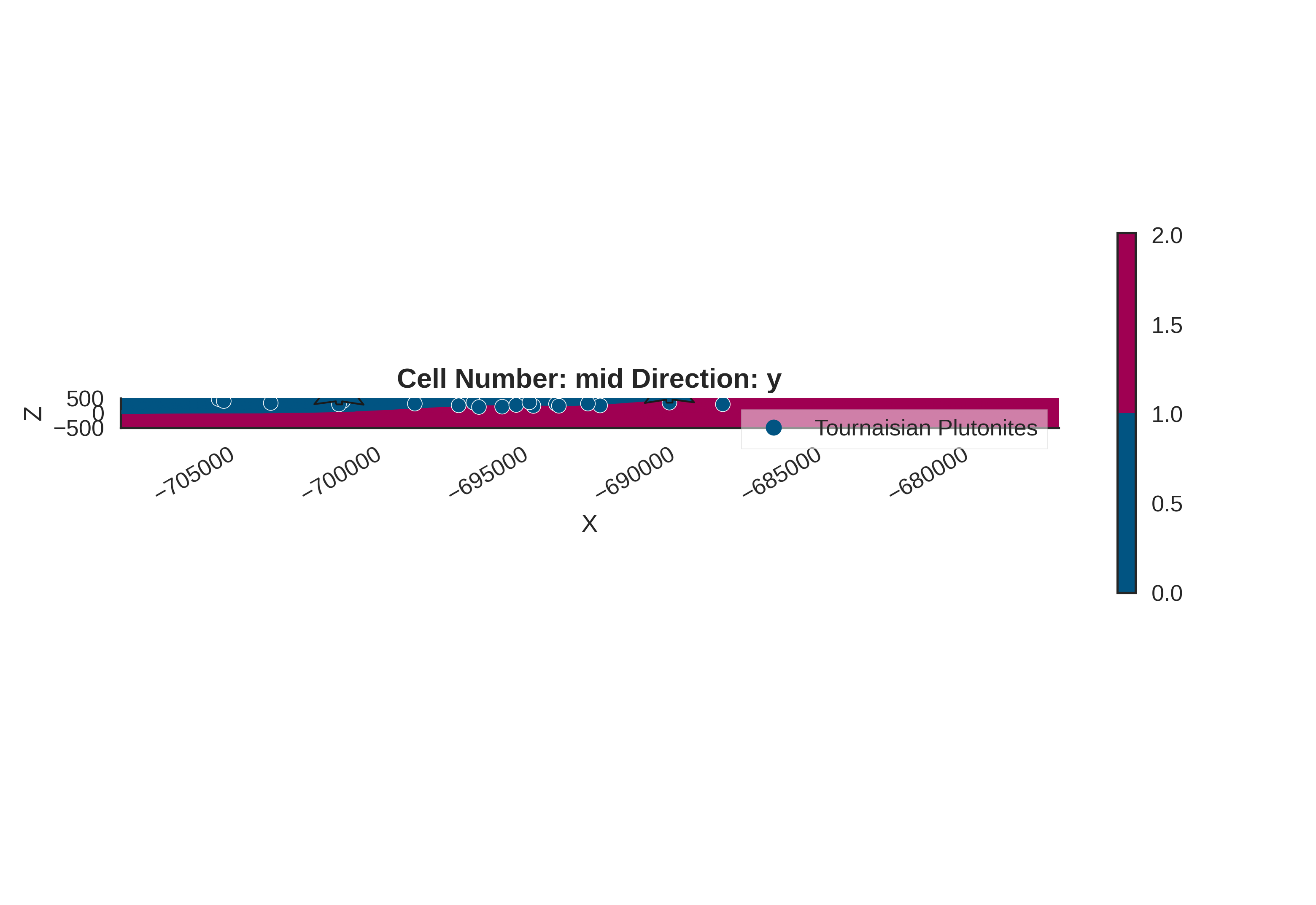
We configure the GemPy geological model to compute gravity at observation locations. The model uses an implicit potential field method to interpolate geological structures from sparse input data (orientations and surface points).

Sigmoid slope parameter: Controls the sharpness of lithological boundaries. Higher values (e.g., 100) create sharper transitions, approximating discontinuous interfaces between rock units. This affects gravity computation since density contrasts are strongest at sharp boundaries.

gp.compute_model(simple_geo_model)
gpv.plot_2d(simple_geo_model)

Setting Backend To: AvailableBackends.PYTORCH
Using sequential processing for 1 surfaces
/home/leguark/.venv/2025/lib/python3.13/site-packages/torch/utils/_device.py:103: UserWarning: Using torch.cross without specifying the dim arg is deprecated.
Please either pass the dim explicitly or simply use torch.linalg.cross.
The default value of dim will change to agree with that of linalg.cross in a future release. (Triggered internally at /pytorch/aten/src/ATen/native/Cross.cpp:63.)
  return func(*args, **kwargs)

<gempy_viewer.modules.plot_2d.visualization_2d.Plot2D object at 0x7f77af35e660>

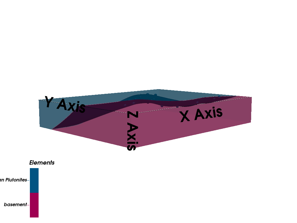
gpv.plot_3d(
    model=simple_geo_model,
    ve=5,
    image=False,
    kwargs_pyvista_bounds={
            'show_xlabels': False,
            'show_ylabels': False,
            'show_zlabels': False,
    }
)

/home/leguark/PycharmProjects/gempy_viewer/gempy_viewer/modules/plot_3d/drawer_surfaces_3d.py:38: PyVistaDeprecationWarning:
../../../gempy_viewer/gempy_viewer/modules/plot_3d/drawer_surfaces_3d.py:38: Argument 'color' must be passed as a keyword argument to function 'BasePlotter.add_mesh'.
From version 0.50, passing this as a positional argument will result in a TypeError.
  gempy_vista.surface_actors[element.name] = gempy_vista.p.add_mesh(

<gempy_viewer.modules.plot_3d.vista.GemPyToVista object at 0x7f77af35da90>

geo_model, xy_ravel = setup_geomodel(gravity_data, simple_geo_model)
geo_model.interpolation_options.sigmoid_slope = 100

print(f"\n✓ Geomodel configured with {len(xy_ravel)} gravity measurement locations")

Setting Backend To: AvailableBackends.PYTORCH
Using actual gravity measurement locations...
Using 20 actual measurement points
Computing forward gravity model...
Setting up centered grid...
Active grids: GridTypes.OCTREE|CENTERED|NONE
Calculating gravity gradient...
Configuring geophysics input...
Active grids: GridTypes.CENTERED|NONE
Setting Backend To: AvailableBackends.PYTORCH

✓ Geomodel configured with 20 gravity measurement locations

Step 3: Compute Baseline Forward Model

The Forward Problem

Before inversion, we compute a forward model with initial (baseline) parameters. This serves multiple purposes:

1. Verify the forward model runs correctly

2. Assess initial fit to observations

3. Establish normalization parameters for the likelihood

The forward gravity computation involves:

1. Interpolating geological structure from control points

2. Assigning densities to each rock unit

3. Computing gravitational attraction at each observation station

4. Accounting for station elevations and 3D geometry

baseline_fw_gravity_np = baseline(geo_model)
print(f"\nBaseline forward gravity:")
print(f"  Range: {baseline_fw_gravity_np.min():.1f} to {baseline_fw_gravity_np.max():.1f} µGal")
print(f"  Mean: {baseline_fw_gravity_np.mean():.1f} µGal")

============================================================
COMPUTING BASELINE FORWARD MODEL
============================================================
Computing gravity with mean/initial prior parameters...
Baseline forward model statistics:
  Mean: 24.52 μGal
  Std:  4.86 μGal
  Min:  8.20 μGal
  Max:  28.58 μGal
============================================================


Baseline forward gravity:
  Range: -28.6 to -8.2 µGal
  Mean: -24.5 µGal

Step 4: Normalize Forward Model to Observations

The Regional-Residual Problem

Gravity data contains both:

• Regional trends: Long-wavelength signals from deep sources (e.g., Moho, crustal thickness)

• Residual anomalies: Short-wavelength signals from shallow geological structures

Since we’re modeling shallow structures, we need to remove regional trends. The normalization step handles this by aligning the forward model to observations using a reference-based approach.

Alignment method: “align_to_reference” finds an optimal offset that minimizes the difference between forward and observed gravity. The extrapolation buffer adds robustness by considering a range of possible offsets.

This normalization is crucial because absolute gravity values depend on reference frames, but gravity anomalies (differences) are what matter for geological interpretation.

norm_params = normalize(
    baseline_fw_gravity_np,
    observed_gravity_ugal,
    method="align_to_reference",
    extrapolation_buffer=0.3
)
print(f"\nNormalization parameters:")
print(f"  Method: {norm_params['method']}")
print(f"  Parameters: {norm_params}")

Computing align_to_reference alignment parameters...
  Alignment params: {'method': 'align_to_reference', 'reference_mean': 25535.6, 'reference_std': 8288.689820472231, 'baseline_forward_mean': -24.516145854322723, 'baseline_forward_std': 4.8571060383169495}

Normalization parameters:
  Method: align_to_reference
  Parameters: {'method': 'align_to_reference', 'reference_mean': 25535.6, 'reference_std': 8288.689820472231, 'baseline_forward_mean': -24.516145854322723, 'baseline_forward_std': 4.8571060383169495}

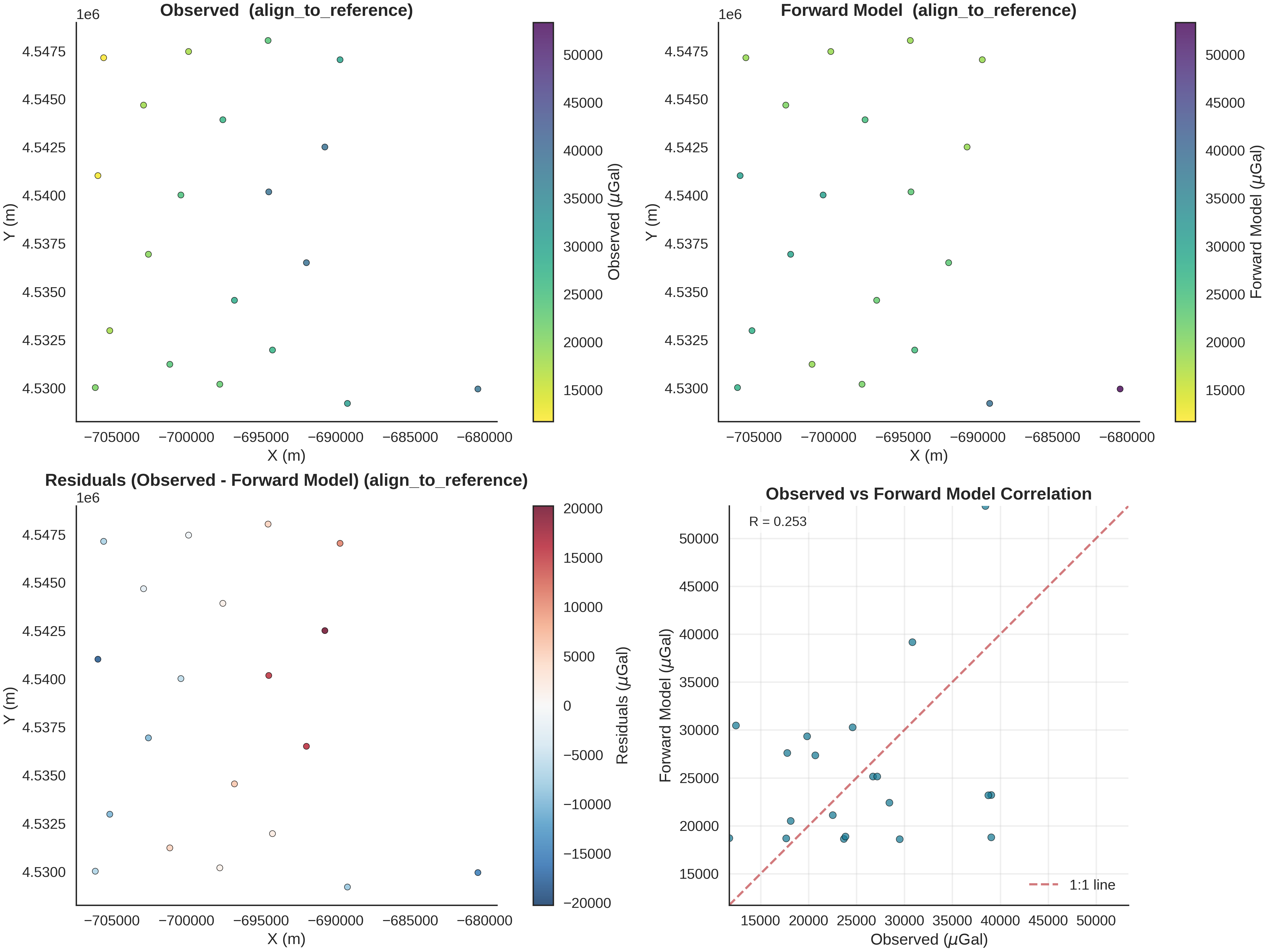
Understanding plot_gravity_comparison

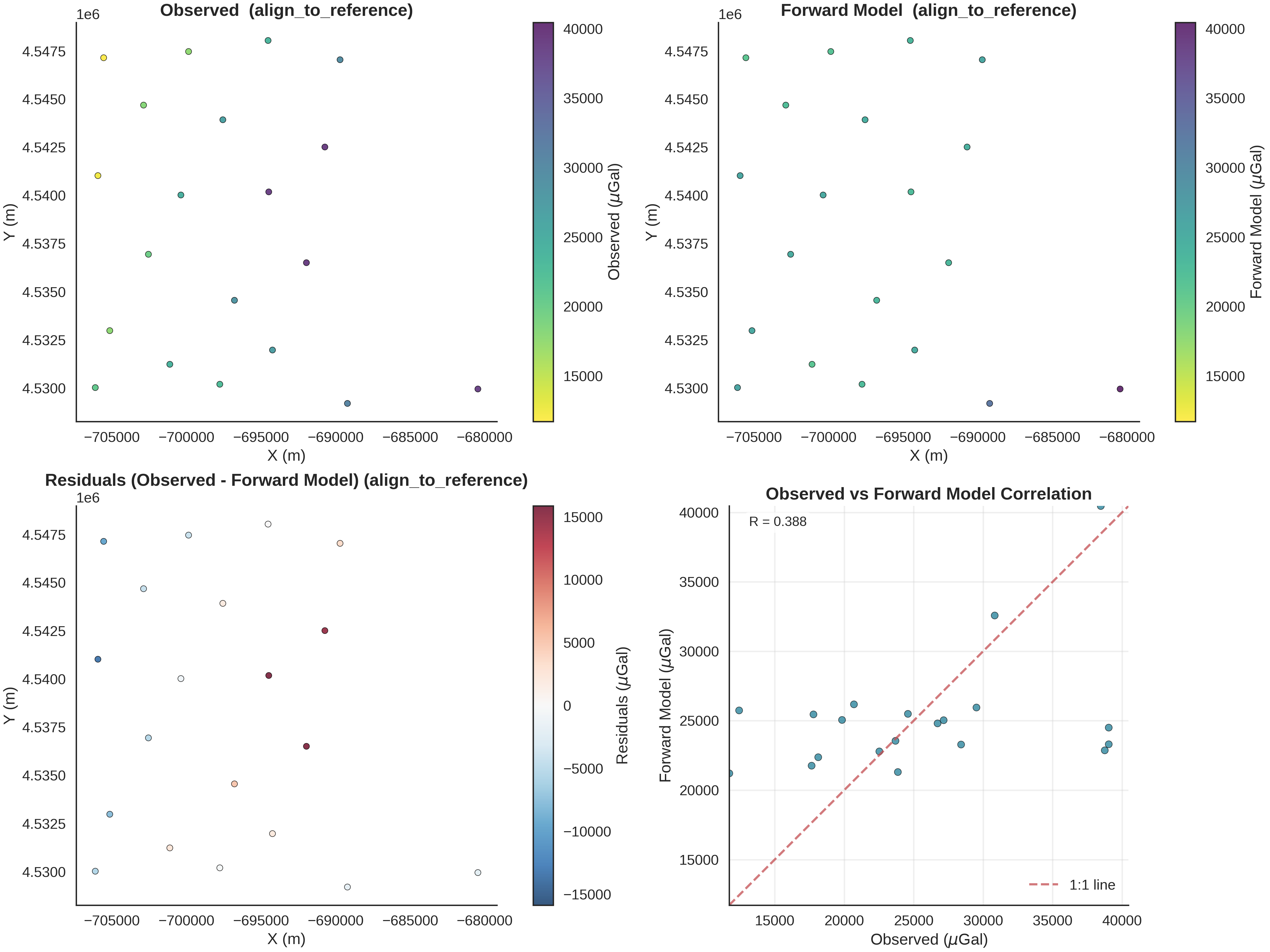
This visualization function creates a comprehensive 4-panel comparison between observed and forward-modeled gravity data:

Panel 1 (Top-Left): Observed Gravity - Shows the spatial distribution of measured gravity values at station locations - Color represents gravity magnitude (viridis_r colormap: dark = high, light = low) - Each point is a measurement station with its x,y coordinates

Panel 2 (Top-Right): Forward Model Gravity - Shows the predicted gravity from our geological model at the same locations - Uses the SAME colorbar limits as Panel 1 for direct visual comparison - Reveals how well our model predicts the spatial patterns

Panel 3 (Bottom-Left): Residuals (Observed - Forward) - Shows the mismatch between observations and predictions - Uses RdBu_r colormap: red = model underpredicts, blue = model overpredicts - Symmetric colorbar centered on zero - Spatial patterns in residuals indicate:

• Systematic errors → model is too simple

• Random scatter → good fit with measurement noise

• Clusters of large residuals → missing geological features

Panel 4 (Bottom-Right): Correlation Plot - Scatter plot: observed (x-axis) vs forward model (y-axis) - Red dashed line: perfect 1:1 agreement - Points on the line = perfect prediction - Correlation coefficient R quantifies linear relationship (-1 to 1) - Interpretation:

• R ≈ 1: excellent fit

• R ≈ 0.7-0.9: good fit with some misfit

• R < 0.5: poor fit, model needs improvement

plot_geophysics_comparison(forward_norm=(align_forward_to_observed(baseline_fw_gravity_np, norm_params)), normalization_method="align_to_reference", observed_ugal=observed_gravity_ugal, xy_ravel=xy_ravel)

Step 5: Define Prior Distributions

Prior Knowledge in Bayesian Inference

Priors encode our geological knowledge before seeing the gravity data. They serve multiple purposes:

1. Regularization: Prevent unphysical parameter values

2. Information integration: Incorporate knowledge from other data sources

3. Computational efficiency: Guide MCMC sampler to high-probability regions

Prior on Dips

We use a Normal distribution to represent our belief about layer orientations:

\[\text{dip} \sim \mathcal{N}(10^\circ,\, 10^\circ)\]

Interpretation:

• Mean (10°): Based on regional geology, we expect shallow-dipping layers (nearly horizontal but with slight tilt)

• Std (10°): Allows for moderate uncertainty (±10° covers range of 0-30°)

• This prior is weakly informative: it guides inference but can be overridden by data

For a more complex model, we would also define priors on densities:

"density": dist.Normal(
    loc=torch.tensor([2.9, 2.3]),  # plutonites, host rock
    scale=torch.tensor(0.15)
).to_event(1)

Where typical crustal densities range from 2.2-3.0 g/cm³.

n_orientations = geo_model.orientations_copy.xyz.shape[0]
prior_key_dips = r'dips'
prior_key_densities = r'density'
model_priors = {
        prior_key_dips     : dist.Normal(
            loc=(torch.ones(n_orientations) * 10.0),
            scale=torch.tensor(10.0, dtype=torch.float64),
            validate_args=True
        ).to_event(1),
        prior_key_densities: dist.Normal(
            loc=(torch.tensor([
                    2.9 - 2.67,  # plutonites
                    2.3 - 2.67  # host
            ])),
            scale=torch.tensor(0.15),
        ).to_event(1)
}

print(f"\nPrior on dips:")
print(f"  Number of orientations: {n_orientations}")
print(f"  Mean: 10°")
print(f"  Std: 10°")

Prior on dips:
  Number of orientations: 2
  Mean: 10°
  Std: 10°

Step 6: Define Deterministic Functions

Tracking Intermediate Quantities

Deterministic functions compute derived quantities during inference. These are not sampled but are deterministic transformations of sampled parameters and model outputs.

We track:

• gravity_response_raw: Unnormalized forward gravity (before alignment)

• gravity_response: Normalized and aligned to observations (used in likelihood)

• mean_gravity / max_gravity: Summary statistics for diagnostics

These deterministics help with:

1. Debugging: Inspect intermediate values if inference fails

2. Visualization: Plot how gravity predictions evolve during sampling

3. Diagnostics: Check if normalized values are reasonable

Step 7: Define Likelihood Function

The Likelihood: Connecting Model to Data

The likelihood quantifies how probable the observed data is given model parameters. It defines the noise model:

\[y_i \sim \mathcal{N}(f_i(θ), σ^2)\]

Where:

• y_i: Observed gravity at station i

• f_i(θ): Forward model prediction at station i

• σ: Measurement noise standard deviation

Diagonal vs Hierarchical Likelihood

We use a diagonal likelihood here (assumes independent noise across stations). For more robust inversion, a hierarchical likelihood can be used:

# Hierarchical: each station has its own noise level
likelihood_fn = generate_multigravity_likelihood_hierarchical_per_station(
    norm_params=norm_params
)

Benefits of hierarchical modeling:

1. Automatic outlier detection: Stations with high σ are downweighted

2. Robustness: Reduces influence of problematic measurements

3. Realism: Different stations have different measurement quality

The hierarchical model estimates per-station noise:

\[\begin{split}σ_i \sim \text{HalfNormal}(τ) \\\\ y_i \sim \mathcal{N}(f_i(θ), σ_i^2)\end{split}\]

Understanding generate_multigravity_likelihood_hierarchical_per_station

This function creates a hierarchical Bayesian likelihood that treats each gravity station’s measurement noise as an unknown parameter to be inferred.

Why hierarchical modeling?

Real gravity data has station-dependent noise due to: - Instrument precision differences - Local environmental conditions (vibrations, temperature) - Terrain corrections quality - Measurement protocol variations

Instead of assuming all stations have identical noise, hierarchical modeling:

1. Estimates noise separately for each station

2. Links stations through shared hyperparameters (partial pooling)

3. Automatically identifies outliers (high-noise stations)

4. Provides robust inference by downweighting problematic data

Mathematical Structure:

The hierarchical model has three levels:

\[\begin{split}\text{Level 1 (Hyperpriors):} \\\\ \mu_{\log\sigma} \sim \mathcal{N}(\log(5000), 0.5) \\\\ \tau_{\log\sigma} \sim \text{HalfNormal}(0.5)\end{split}\]

\[\begin{split}\text{Level 2 (Station-specific noise):} \\\\ \log(\sigma_i) \sim \mathcal{N}(\mu_{\log\sigma}, \tau_{\log\sigma})\end{split}\]

\[\begin{split}\text{Level 3 (Observations):} \\\\ y_i \sim \mathcal{N}(f_i(\theta), \sigma_i^2)\end{split}\]

Parameter Interpretation:

• μ_log_σ: Global mean noise level (log scale)

  • Prior centered at log(5000) ≈ 8.5, meaning typical noise is ~5000 µGal

  • Uncertainty of 0.5 allows 1σ range of [3000, 8200] µGal

• τ_log_σ: Variability between stations (log scale)

  • HalfNormal(0.5) prior: most stations similar, but allows outliers

  • Small τ → stations have similar noise (strong pooling)

  • Large τ → stations have very different noise (weak pooling)

• σ_i: Each station’s noise standard deviation

  • Inferred from data automatically

  • High σ_i → station is an outlier or has poor data quality

  • Low σ_i → station is reliable

Benefits over fixed noise:

1. Robustness: Outliers get high σ_i and are downweighted automatically

2. Adaptivity: Model learns which stations to trust

3. Uncertainty quantification: Know which measurements are reliable

4. No manual outlier removal: Statistical approach to data quality

Working with log-scale:

We model log(σ) rather than σ directly because:

• Noise must be positive: exp(log σ) > 0 always

• More symmetric uncertainty: equal probability of σ/2 and 2σ

• Numerically stable for optimization and sampling

Partial pooling effect:

The hierarchical structure provides “partial pooling” between no pooling (each station independent) and complete pooling (all stations identical):

• Stations with few observations borrow strength from others (shrinkage)

• Stations with many observations stay close to their data

• Automatically balances individual evidence vs. group information

likelihood_fn = generate_multigravity_likelihood_hierarchical_per_station(
    norm_params=norm_params
)

print("✓ Likelihood function created (hierarchical per-station)")
print(f"  Global mean noise prior: ~5000.0 µGal")
print(f"  Each station's noise will be inferred from data")

✓ Likelihood function created (hierarchical per-station)
  Global mean noise prior: ~5000.0 µGal
  Each station's noise will be inferred from data

Inspecting the Likelihood Function Source Code

To fully understand what the likelihood function does internally, we can inspect its source code. This is particularly useful because the likelihood is the most variable component across different inversions - it defines how model predictions connect to observations and what noise model is assumed.

The source code reveals:

• How simulated geophysics is aligned to observations

• What Pyro distributions are used for the noise model

• Which parameters are sampled (inferred) vs fixed

• The hierarchical structure (hyperpriors → station-level parameters → observations)

import inspect

print("\n" + "=" * 70)
print("LIKELIHOOD FUNCTION SOURCE CODE")
print("=" * 70)
print(inspect.getsource(generate_multigravity_likelihood_hierarchical_per_station))
print("=" * 70)

======================================================================
LIKELIHOOD FUNCTION SOURCE CODE
======================================================================
def generate_multigravity_likelihood_hierarchical_per_station(norm_params):
    """
    Per-station noise with hierarchical structure.
    Best for: Different stations with unknown individual noise levels.
    """

    def likelihood_fn(solutions: gp.data.Solutions) -> dist.Distribution:
        simulated_geophysics = align_forward_to_observed(-solutions.gravity, norm_params)
        pyro.deterministic(r'$\mu_{gravity}$', simulated_geophysics.detach())
        n_stations = simulated_geophysics.shape[0]

        # Global hyperprior on typical noise level
        mu_log_sigma = pyro.sample(
            "mu_log_sigma",
            dist.Normal(
                torch.tensor(np.log(5000.0), dtype=torch.float64),
                torch.tensor(0.5, dtype=torch.float64)
            )
        )

        # How much stations vary from each other
        tau_log_sigma = pyro.sample(
            "tau_log_sigma",
            dist.HalfNormal(torch.tensor(0.5, dtype=torch.float64))
        )

        # Per-station noise (centered on global mean)
        log_sigma_stations = pyro.sample(
            "log_sigma_stations",
            dist.Normal(
                mu_log_sigma.expand([n_stations]),
                tau_log_sigma
            ).to_event(1)
        )

        sigma_stations = torch.exp(log_sigma_stations)
        pyro.deterministic("sigma_stations", sigma_stations)

        return dist.Normal(simulated_geophysics, sigma_stations).to_event(1)

    return likelihood_fn

======================================================================

Step 8: Create Probabilistic Model

Building the Full Bayesian Model

We now combine all components into a Pyro probabilistic model. This orchestrates the inference workflow:

1. Sample from priors (dips, densities)

2. Update GeoModel via set_interp_input_fn

3. Run forward gravity computation

4. Compute deterministics (tracked quantities)

5. Evaluate likelihood against observations

The `set_interp_input_fn` function

This function bridges Pyro’s sampled parameters to GemPy’s geological model. The actual implementation (set_priors) performs these steps:

def set_priors(samples: dict, geo_model: gp.data.GeoModel):
    # 1. Create interpolation input from current model state
    interp_input = interpolation_input_from_structural_frame(geo_model)

    # 2. Extract current orientation gradients
    og_gradients = interp_input.orientations.dip_gradients

    # 3. Compute azimuth, dip, polarity from gradients
    azimuth, dip, polarity = compute_adp_from_gradients(
        G_x=og_gradients[:, 0],
        G_y=og_gradients[:, 1],
        G_z=og_gradients[:, 2]
    )

    # 4. Replace dip with sampled values, keeping azimuth/polarity
    sampled_dips = samples["dips"]
    new_gradients = convert_orientation_to_pole_vector(
        azimuth=azimuth,
        dip=sampled_dips,  # ← This is what we're inferring
        polarity=polarity
    )

    # 5. Update interpolation input with new gradients
    interp_input.orientations.dip_gradients = new_gradients

    # 6. Update densities
    geo_model.geophysics_input.densities = samples["density"]

    return interp_input

Why this complexity?

GemPy internally represents orientations as 3D gradient vectors (G_x, G_y, G_z), not as angles. The conversion ensures:

• Sampled dip angles are properly transformed to gradients

• Azimuth and polarity remain consistent with original data

• All operations are differentiable (required for NUTS)

This coupling allows MCMC to explore geological parameter space while computing physically-consistent gravity responses.

Understanding make_gempy_pyro_model_extended

This function creates a complete Bayesian probabilistic model by connecting all the pieces we’ve defined. It orchestrates the entire inference workflow within Pyro’s probabilistic programming framework.

Function Arguments Explained:

1. priors (dict): Prior distributions for all parameters - Keys: parameter names (e.g., “dips”, “density”) - Values: Pyro distribution objects - These encode our geological knowledge before seeing data

2. set_interp_input_fn (callable): Bridge between Pyro and GemPy - Takes sampled parameters from Pyro - Updates the GemPy geological model accordingly - Returns modified InterpolationInput for forward modeling - Example: set_priors() updates orientations and densities

3. likelihood_fn (callable): Connects predictions to observations - Takes GemPy Solutions (forward model output) - Returns Pyro distribution representing p(data|parameters) - Defines the noise model (Gaussian, Student-t, etc.)

4. pre_forward_deterministics (dict): Quantities tracked BEFORE forward model - Useful for debugging parameter transformations - Example: track transformed coordinates, scaled parameters

5. post_forward_deterministics (dict): Quantities tracked AFTER forward model - Monitor derived quantities during inference - Keys: variable names for ArviZ - Values: functions that extract/compute quantities from Solutions - Example: track mean gravity, max gravity, normalized response

6. obs_name (str): Name for observed data in ArviZ output - Used for labeling in posterior predictive plots - Helps identify which likelihood corresponds to which data

What happens inside make_gempy_pyro_model_extended?

The function creates a Pyro model that executes this sequence on each MCMC iteration:

1. Sample parameters from priors:
   θ ~ p(θ)
   Example: dips ~ Normal(10, 10)

2. Transform parameters via set_interp_input_fn:
   InterpolationInput = set_priors(θ, geo_model)
   Updates: orientations.dip, densities, etc.

3. Compute pre-forward deterministics (if any):
   pyro.deterministic("param_squared", θ**2)

4. Run GemPy forward model:
   Solutions = gp.compute_model(geo_model)
   Computes: gravity field at observation points

5. Compute post-forward deterministics:
   pyro.deterministic("gravity_response", normalize(Solutions.gravity))
   pyro.deterministic("mean_gravity", torch.mean(...))

6. Evaluate likelihood:
   y_obs ~ likelihood_fn(Solutions)
   Computes: log p(y_obs | θ)

7. MCMC/VI uses log p(y_obs | θ) + log p(θ) to update sampler

Why this architecture?

• Modularity: Each component (prior, forward model, likelihood) can be modified independently

• Flexibility: Easy to add new parameters, change noise models, or incorporate multiple data types

• Automatic differentiation: Pyro tracks gradients through the entire workflow, enabling efficient NUTS sampling

• Diagnostics: Deterministics provide visibility into intermediate steps without affecting inference

Return value:

A GemPyPyroModel object that can be passed to: - gpp.run_nuts_inference() for MCMC sampling - gpp.run_predictive() for prior/posterior predictive checks - gpp.run_vi_inference() for variational inference (faster approximation)

prob_model: gpp.GemPyPyroModel = gpp.make_gempy_pyro_model(
    priors=model_priors,
    set_interp_input_fn=set_priors,
    likelihood_fn=likelihood_fn,
    obs_name="Gravity Measurement"
)

print("✓ Probabilistic model created")
print("  Model components:")
print("    - Priors: dips (orientations), densities")
print("    - Forward model: GemPy geological interpolation + gravity")
print("    - Likelihood: Hierarchical per-station noise")
print("    - Deterministics: gravity_response, mean_gravity, max_gravity")

Setting Backend To: AvailableBackends.PYTORCH
✓ Probabilistic model created
  Model components:
    - Priors: dips (orientations), densities
    - Forward model: GemPy geological interpolation + gravity
    - Likelihood: Hierarchical per-station noise
    - Deterministics: gravity_response, mean_gravity, max_gravity

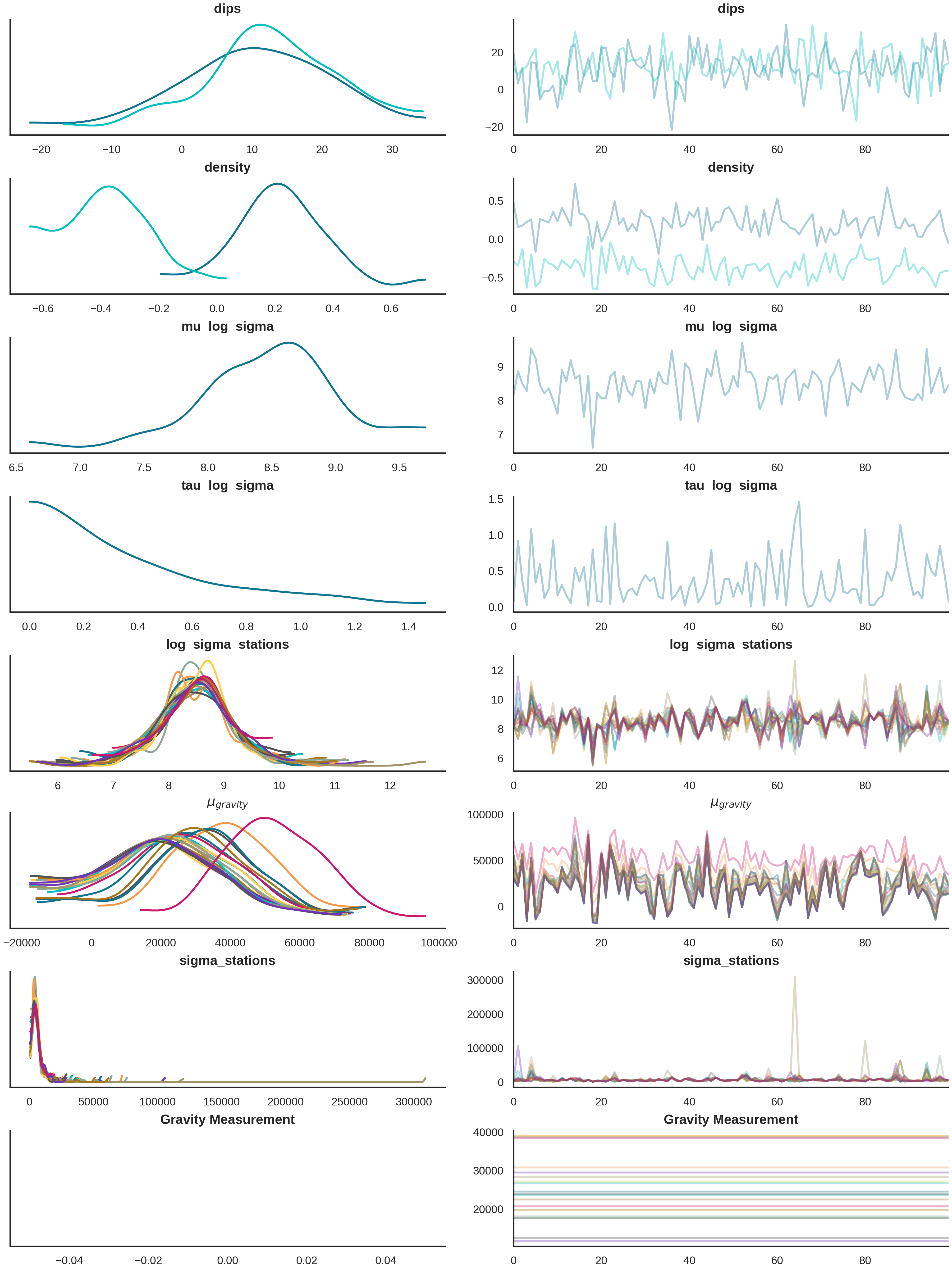
Step 9: Prior Predictive Checks

Why Prior Predictive Checks?

Before running inference, we sample from the prior to answer critical questions:

1. Range check: Do prior predictions cover the observed values? If not, the prior may be too restrictive or the model inadequate.

2. Model adequacy: Can any parameter combination explain the data? If prior predictions are far from observations, we may need:

   • More model complexity (additional parameters)

   • Different physics (e.g., include magnetics, seismic)

   • Revised priors (incorrect geological assumptions)

3. Prior sensitivity: How much do predictions vary under the prior? High variability indicates the prior is uninformative; low variability suggests the prior is too restrictive.

Expected behavior:

In this test case, we simulate 20 observations per iteration. Some forward models explain certain stations well but fail at others, suggesting:

• The model may be oversimplified

• Some stations could be outliers

• Additional data types might not help without increasing model complexity

Prior predictive sampling generates data as if we hadn’t seen the observations yet.

print("\nRunning prior predictive sampling (100 samples)...")
prior_inference_data: az.InferenceData = gpp.run_predictive(
    prob_model=prob_model,
    geo_model=geo_model,
    y_obs_list=torch.tensor(observed_gravity_ugal),
    n_samples=100,
    plot_trace=True
)

print("✓ Prior predictive sampling complete")

Running prior predictive sampling (100 samples)...
/home/leguark/.venv/2025/lib/python3.13/site-packages/arviz/stats/density_utils.py:488: UserWarning: Your data appears to have a single value or no finite values
  warnings.warn("Your data appears to have a single value or no finite values")
✓ Prior predictive sampling complete

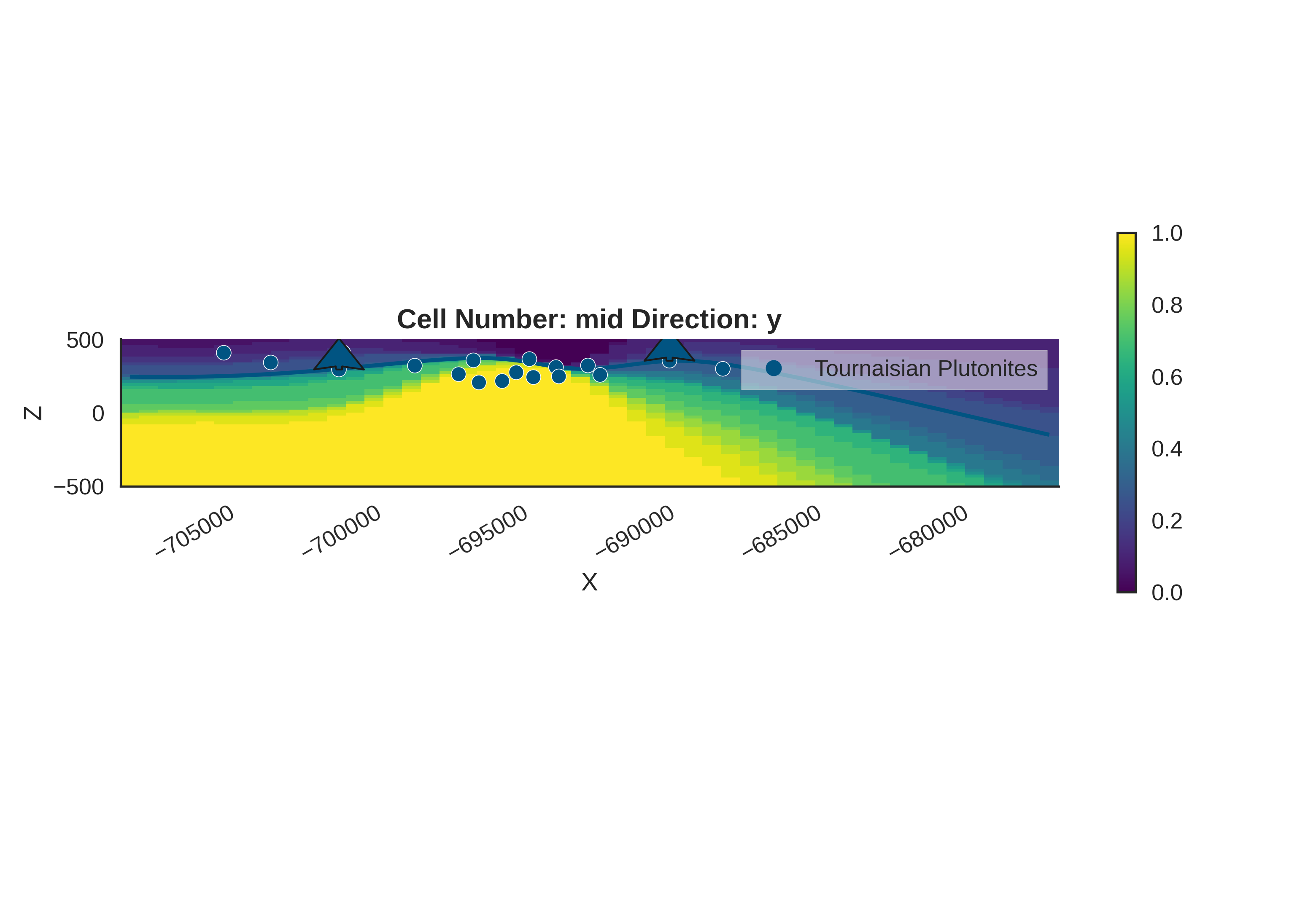
Visualize Prior Geological Models

Understanding gempy_viz

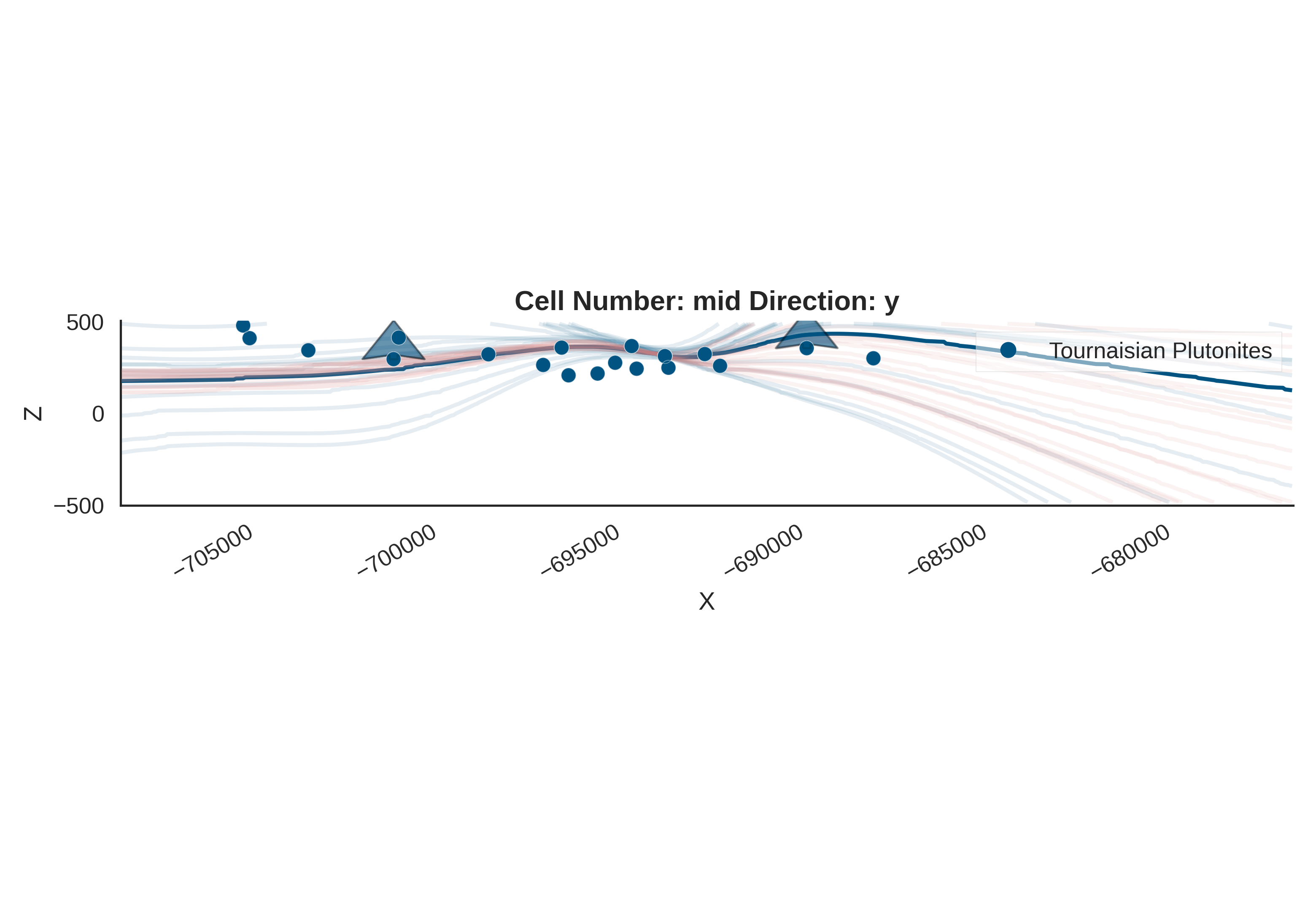
This function creates a 2D cross-section visualization showing:

1. The geological model: Interpolated lithological boundaries

2. Prior uncertainty via KDE (Kernel Density Estimation):

   • Background colored contours show probability density of boundary locations

   • Darker/more saturated colors = higher probability

   • Shows where the geological boundary is likely to be given our prior beliefs

3. Representative realizations: Individual model samples overlaid as contours

Why visualize the prior?

• Verify that prior predictions span a geologically reasonable range

• Check if the model can produce diverse enough structures

• Identify if priors are too restrictive (narrow KDE) or too vague (very wide KDE)

KDE interpretation:

• Narrow, focused density: Strong prior belief about structure location

• Wide, diffuse density: High uncertainty in structure location

• Multiple modes: Prior suggests multiple possible configurations

gempy_viz(
    geo_model=geo_model,
    prior_inference_data=prior_inference_data,
    n_samples=20
)

Active grids: GridTypes.OCTREE|NONE
Setting Backend To: AvailableBackends.PYTORCH
Setting Backend To: AvailableBackends.PYTORCH
/home/leguark/PycharmProjects/gempy_viewer/gempy_viewer/modules/plot_2d/drawer_contours_2d.py:38: UserWarning: The following kwargs were not used by contour: 'linewidth', 'contour_colors'
  contour_set = ax.contour(
Setting Backend To: AvailableBackends.PYTORCH
Setting Backend To: AvailableBackends.PYTORCH
Setting Backend To: AvailableBackends.PYTORCH
Setting Backend To: AvailableBackends.PYTORCH
Setting Backend To: AvailableBackends.PYTORCH
Setting Backend To: AvailableBackends.PYTORCH
Setting Backend To: AvailableBackends.PYTORCH
Setting Backend To: AvailableBackends.PYTORCH
Setting Backend To: AvailableBackends.PYTORCH
Setting Backend To: AvailableBackends.PYTORCH
Setting Backend To: AvailableBackends.PYTORCH
Setting Backend To: AvailableBackends.PYTORCH
Setting Backend To: AvailableBackends.PYTORCH
Setting Backend To: AvailableBackends.PYTORCH
Setting Backend To: AvailableBackends.PYTORCH
Setting Backend To: AvailableBackends.PYTORCH
Setting Backend To: AvailableBackends.PYTORCH
Setting Backend To: AvailableBackends.PYTORCH
Setting Backend To: AvailableBackends.PYTORCH

<gempy_viewer.modules.plot_2d.visualization_2d.Plot2D object at 0x7f77af26e990>

Compare Multiple Prior Predictions to Observations

Understanding plot_many_observed_vs_forward

This diagnostic plot shows how well different prior samples fit the data. It helps answer: “Can ANY model from our prior explain the observations?”

Plot Structure:

• X-axis: Observed gravity (sorted by value for clarity)

• Y-axis: Forward-modeled gravity from different prior samples

• Each colored line: One realization from the prior distribution

• Red dashed line: Perfect 1:1 agreement

What to look for:

1. Lines parallel to 1:1: Model captures the overall trend

   • Offset from 1:1 is handled by normalization

   • Slope matters: should be close to 1.0

2. Lines crossing each other: Different models fit different subsets of data

   • Some samples fit low-gravity stations well

   • Other samples fit high-gravity stations well

   • Suggests parameter trade-offs or model inadequacy

3. All lines far from 1:1: Prior may be mis-specified

   • Models can’t explain observations

   • Need to adjust priors or add model complexity

4. Lines bunched together: Prior is restrictive

   • Limited parameter range

   • May need wider priors for exploration

Implications for inference:

• If some lines pass through observations → posterior will identify those parameters

• If NO lines match observations → model structure is inadequate

• Scatter in lines → posterior will reduce uncertainty by selecting best-fitting models

plot_many_observed_vs_forward(
    forward_norm=(align_forward_to_observed(baseline_fw_gravity_np, norm_params)),
    many_forward_norm=prior_inference_data.prior[r'$\mu_{gravity}$'].values[0, -10:],
    observed_norm=observed_gravity_ugal,
    unit_label='μGal'
)

Step 10: Run MCMC Inference with NUTS

MCMC and the NUTS Algorithm

Markov Chain Monte Carlo (MCMC) is a family of algorithms for sampling from probability distributions. We use the No-U-Turn Sampler (NUTS), a variant of Hamiltonian Monte Carlo (HMC) that:

1. Uses gradient information: Computes ∇log p(θ|y) to efficiently explore high-dimensional parameter space

2. Adapts automatically: No manual tuning of trajectory length

3. Provides diagnostics: Divergences, tree depth, and acceptance rates indicate sampling quality

How NUTS Works

NUTS simulates Hamiltonian dynamics to propose new parameter values:

1. Start at current parameter θ

2. Introduce momentum variable p ~ Normal(0, M)

3. Simulate Hamilton’s equations using leapfrog integration

4. Build a binary tree of candidate states

5. Stop when trajectory makes a “U-turn” (starts returning)

6. Select new state from tree with probability proportional to posterior

Configuration Parameters

• step_size (0.0001): Small steps for careful exploration of posterior. Too large → many rejections; too small → slow mixing.

• adapt_step_size (True): Automatically tune step size during warmup to achieve target acceptance probability.

• target_accept_prob (0.65): Aim for 65% acceptance rate. Lower values (e.g., 0.6) → larger steps, faster exploration, more rejections. Higher values (e.g., 0.9) → smaller steps, better for difficult posteriors.

• max_tree_depth (5): Computational budget per iteration. Each depth doubles the number of gradient evaluations (2^5 = 32 max). Increase if you see “reached max tree depth” warnings.

• init_strategy (‘median’): Start chains at median of prior. Alternatives: ‘uniform’ (random from prior), custom initial values.

• num_samples (200): Number of posterior samples after warmup. More samples → better posterior approximation but slower.

• warmup_steps (200): Number of iterations to tune sampler. During warmup, NUTS adapts step size and mass matrix. Samples are discarded.

• num_chains (1): Number of independent MCMC chains. Multiple chains help diagnose convergence (R-hat statistic) but are computationally expensive.

Outputs

• data.posterior: Parameter samples (dips, densities)

• data.posterior_predictive: Forward gravity predictions from posterior

• data.sample_stats: Diagnostics (divergences, tree depth, acceptance rate)

print("\nRunning NUTS inference...")
print("  Warmup: 200 steps")
print("  Sampling: 200 samples")
print("  Chains: 1")

RUN_SIMULATION = False
if RUN_SIMULATION:
    data = gpp.run_nuts_inference(
        prob_model=prob_model,
        geo_model=geo_model,
        y_obs_list=torch.tensor(observed_gravity_ugal),
        config=NUTSConfig(
            step_size=0.0001,
            adapt_step_size=True,
            target_accept_prob=0.65,
            max_tree_depth=5,
            init_strategy='median',
            num_samples=200,
            warmup_steps=200,
        ),
        plot_trace=True,
        run_posterior_predictive=True
    )

    print("✓ NUTS inference complete")

    # Combine Prior and Posterior
    # ----------------------------
    #
    # For comparison and diagnostics, we store both prior and posterior in the same
    # ArviZ InferenceData object. This allows us to visualize how our beliefs changed
    # after seeing the data.

    data.extend(prior_inference_data)
    print("✓ Prior and posterior combined")

    data.to_netcdf(os.path.join(os.path.dirname(__file__), "New Grav"))

else:

    from pathlib import Path
    import inspect

    # Get the directory of the current file using inspect
    current_dir = Path(inspect.getfile(inspect.currentframe())).parent.resolve()
    data_path = current_dir / "arviz_data_grav_feb2026.nc"

    if not data_path.exists():
        raise FileNotFoundError(
            f"Data file not found at {data_path}. "
            f"Please run the simulation first with RUN_SIMULATION=True"
        )

    # Read the data file
    data = az.from_netcdf(str(data_path))

Running NUTS inference...
  Warmup: 200 steps
  Sampling: 200 samples
  Chains: 1

Interactive: Pre-computed Results

Running full MCMC chains can be computationally expensive. For convenience, pre-computed .nc files (ArviZ InferenceData) are available for download.

To use them: 1. Download arviz_data_04.nc from the project repository. 2. Place it in the same directory as this script. 3. Set RUN_SIMULATION = False to load the results instantly.

Analysis: Parameter Posterior Statistics

Interpreting the Posterior

The posterior distribution represents our updated beliefs about parameters after seeing the gravity data. Key questions:

1. Did we learn from the data? Compare posterior std to prior std. Posterior should be narrower (more certain).

2. Did beliefs shift? Compare posterior mean to prior mean. Shift indicates data provided information.

3. Are parameters well-constrained? Small posterior std → data strongly constrains parameter. Large posterior std → parameter remains uncertain (weak data signal).

Posterior concentration

The posterior concentrates around models that maximize the number of explained observations. This acts like robust regression: outliers (potentially interesting geological anomalies) may remain unexplained if they conflict with the majority of data.

posterior_dips = data.posterior['dips'].values
print(f"\nPosterior dip statistics:")
print(f"  Shape: {posterior_dips.shape}")
print(f"  Mean: {posterior_dips.mean():.2f}°")
print(f"  Std: {posterior_dips.std():.2f}°")
print(f"  Median: {np.median(posterior_dips):.2f}°")

prior_dips = data.prior['dips'].values
print(f"\nPrior dip statistics:")
print(f"  Mean: {prior_dips.mean():.2f}°")
print(f"  Std: {prior_dips.std():.2f}°")

# Quantify learning
uncertainty_reduction = (1 - posterior_dips.std() / prior_dips.std()) * 100
print(f"\nUncertainty reduction: {uncertainty_reduction:.1f}%")

Posterior dip statistics:
  Shape: (1, 200, 2)
  Mean: 3.94°
  Std: 9.56°
  Median: 3.87°

Prior dip statistics:
  Mean: 11.48°
  Std: 10.03°

Uncertainty reduction: 4.7%

Analysis: Predictive Performance

Posterior Predictive Checks

We compare posterior predictions to observations to assess model fit:

Residual analysis:

• Mean residual ≈ 0: Unbiased model (no systematic over/under-prediction)

• RMS residual: Root-mean-square error quantifies overall misfit

• Residual patterns: Spatial patterns indicate unmodeled geology

What if fit is poor?

If RMS residuals are large compared to expected measurement noise:

1. Model inadequacy: Need more complexity (additional layers, spatial density variations, 3D structure)

2. Wrong physics: May need different geophysical methods

3. Data issues: Outliers, measurement errors, incorrect corrections

posterior_gravity = data.posterior_predictive['Gravity Measurement'].values
print(f"\nPosterior predictive gravity:")
print(f"  Shape: {posterior_gravity.shape}")
print(f"  Mean: {posterior_gravity.mean():.1f} µGal")
print(f"  Std: {posterior_gravity.std():.1f} µGal")

print(f"\nObserved gravity:")
print(f"  Mean: {observed_gravity_ugal.mean():.1f} µGal")
print(f"  Std: {observed_gravity_ugal.std():.1f} µGal")

residuals = posterior_gravity.mean(axis=(0, 1)) - observed_gravity_ugal
print(f"\nResiduals (posterior mean - observed):")
print(f"  Mean: {residuals.mean():.2f} µGal (bias)")
print(f"  RMS: {np.sqrt((residuals ** 2).mean()):.2f} µGal (fit quality)")
print(f"  Max absolute: {np.abs(residuals).max():.2f} µGal")

Posterior predictive gravity:
  Shape: (1, 200, 20)
  Mean: 25535.6 µGal
  Std: 8288.7 µGal

Observed gravity:
  Mean: 25535.6 µGal
  Std: 8288.7 µGal

Residuals (posterior mean - observed):
  Mean: 0.00 µGal (bias)
  RMS: 0.00 µGal (fit quality)
  Max absolute: 0.00 µGal

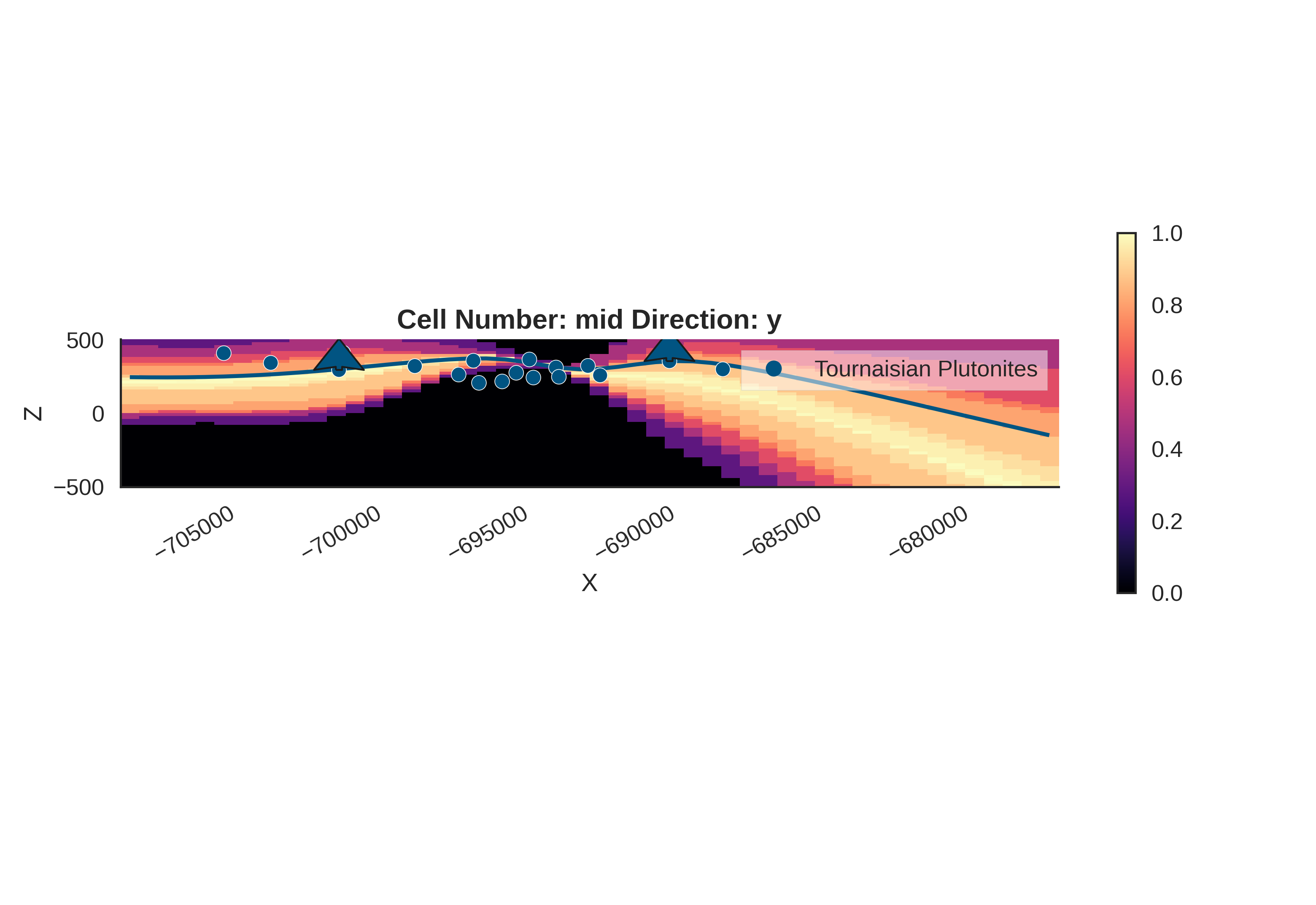
Posterior Predictive: Model Fit Analysis

Understanding Posterior Convergence

In the plot_many_observed_vs_forward visualization, we observe that no single model can perfectly explain all observations simultaneously. This reveals an important aspect of Bayesian inference: the posterior distribution identifies models that best balance the fit across all measurement stations.

What the inference is doing:

The MCMC sampler finds parameter combinations that bring the maximum number of observations close to their measured values. Rather than perfectly fitting a subset of stations, the posterior concentrates on models that provide reasonable explanations across the entire dataset. This “compromise” solution is mathematically optimal under our likelihood model.

Geometric constraints from data:

Even with this distributed fit, the gravity data significantly constrains the possible geological configurations. As visualized in gempy_viz, the posterior distribution shows much tighter bounds on structural geometry than the prior. The inference has successfully ruled out large regions of parameter space that are inconsistent with observations.

Implications:

• Stations that remain poorly fit may indicate localized geological complexity not captured by our current model structure

• The spread in posterior predictions quantifies irreducible uncertainty given model assumptions

• Future model refinements (additional layers, spatially-varying densities) could improve station-by-station fit while maintaining these geometric constraints

plot_many_observed_vs_forward(
    forward_norm=(align_forward_to_observed(baseline_fw_gravity_np, norm_params)),
    many_forward_norm=data.posterior_predictive[r'$\mu_{gravity}$'].values[0, -20:],
    observed_norm=observed_gravity_ugal,
    unit_label='μGal'
)

az.plot_density(
    data=[data, data.prior],
    var_names=["dips", "density"],
    filter_vars="like",
    hdi_prob=0.9999,
    shade=.2,
    data_labels=["Posterior", "Prior"],
    colors=[default_red, default_blue],
)

array([[<Axes: title={'center': 'density\n0'}>,
        <Axes: title={'center': 'density\n1'}>,
        <Axes: title={'center': 'dips\n0'}>],
       [<Axes: title={'center': 'dips\n1'}>, <Axes: >, <Axes: >]],
      dtype=object)

gempy_viz(
    geo_model=geo_model,
    prior_inference_data=data,
    n_samples=20
)

Active grids: GridTypes.OCTREE|NONE
Setting Backend To: AvailableBackends.PYTORCH
Setting Backend To: AvailableBackends.PYTORCH
/home/leguark/PycharmProjects/gempy_viewer/gempy_viewer/modules/plot_2d/drawer_contours_2d.py:38: UserWarning: The following kwargs were not used by contour: 'linewidth', 'contour_colors'
  contour_set = ax.contour(
Setting Backend To: AvailableBackends.PYTORCH
Setting Backend To: AvailableBackends.PYTORCH
Setting Backend To: AvailableBackends.PYTORCH
Setting Backend To: AvailableBackends.PYTORCH
Setting Backend To: AvailableBackends.PYTORCH
Setting Backend To: AvailableBackends.PYTORCH
Setting Backend To: AvailableBackends.PYTORCH
Setting Backend To: AvailableBackends.PYTORCH
Setting Backend To: AvailableBackends.PYTORCH
Setting Backend To: AvailableBackends.PYTORCH
Setting Backend To: AvailableBackends.PYTORCH
Setting Backend To: AvailableBackends.PYTORCH
Setting Backend To: AvailableBackends.PYTORCH
Setting Backend To: AvailableBackends.PYTORCH
Setting Backend To: AvailableBackends.PYTORCH
Setting Backend To: AvailableBackends.PYTORCH
Setting Backend To: AvailableBackends.PYTORCH
Setting Backend To: AvailableBackends.PYTORCH
Setting Backend To: AvailableBackends.PYTORCH
Setting Backend To: AvailableBackends.PYTORCH
Setting Backend To: AvailableBackends.PYTORCH
Setting Backend To: AvailableBackends.PYTORCH
Setting Backend To: AvailableBackends.PYTORCH
Setting Backend To: AvailableBackends.PYTORCH
Setting Backend To: AvailableBackends.PYTORCH
Setting Backend To: AvailableBackends.PYTORCH
Setting Backend To: AvailableBackends.PYTORCH
Setting Backend To: AvailableBackends.PYTORCH
Setting Backend To: AvailableBackends.PYTORCH
Setting Backend To: AvailableBackends.PYTORCH
Setting Backend To: AvailableBackends.PYTORCH
Setting Backend To: AvailableBackends.PYTORCH
Setting Backend To: AvailableBackends.PYTORCH
Setting Backend To: AvailableBackends.PYTORCH
Setting Backend To: AvailableBackends.PYTORCH
Setting Backend To: AvailableBackends.PYTORCH
Setting Backend To: AvailableBackends.PYTORCH
Setting Backend To: AvailableBackends.PYTORCH
Setting Backend To: AvailableBackends.PYTORCH

<gempy_viewer.modules.plot_2d.visualization_2d.Plot2D object at 0x7f778c38d450>

plot_geophysics_comparison(forward_norm=data.prior[r'$\mu_{gravity}$'].mean(axis=1), normalization_method='align_to_reference', observed_ugal=observed_gravity_ugal, xy_ravel=xy_ravel)

plot_geophysics_comparison(forward_norm=data.posterior_predictive[r'$\mu_{gravity}$'].mean(axis=1), normalization_method='align_to_reference', observed_ugal=observed_gravity_ugal, xy_ravel=xy_ravel)

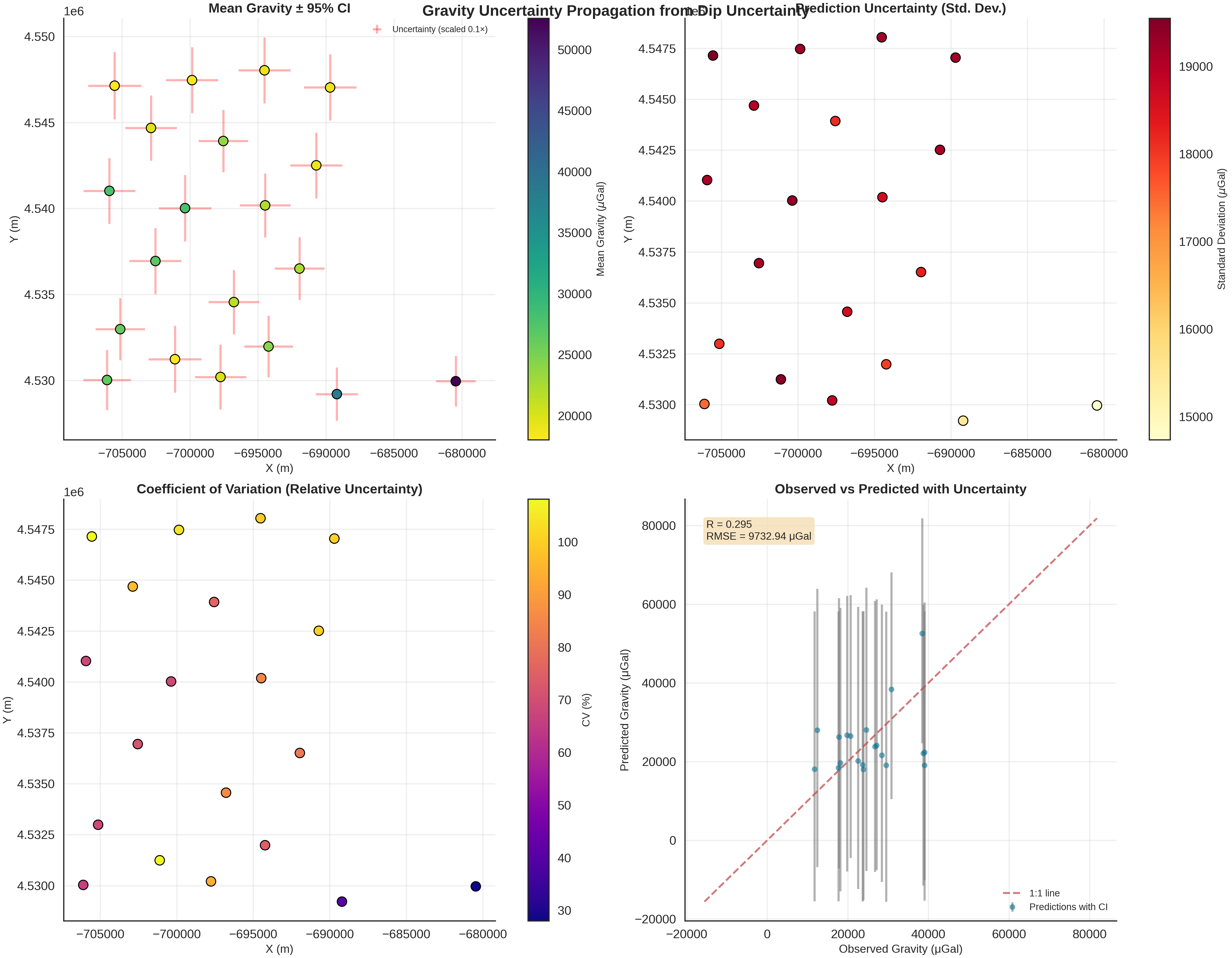
gravity_samples_norm, unit_label = generate_gravity_uncertainty_plots(
    gravity_samples_norm=data.prior[r'$\mu_{gravity}$'].values[0, :],  # (n_samples, n_devices)
    observed_gravity_ugal=observed_gravity_ugal,
    xy_ravel=xy_ravel
)

• 
• 
• 

============================================================
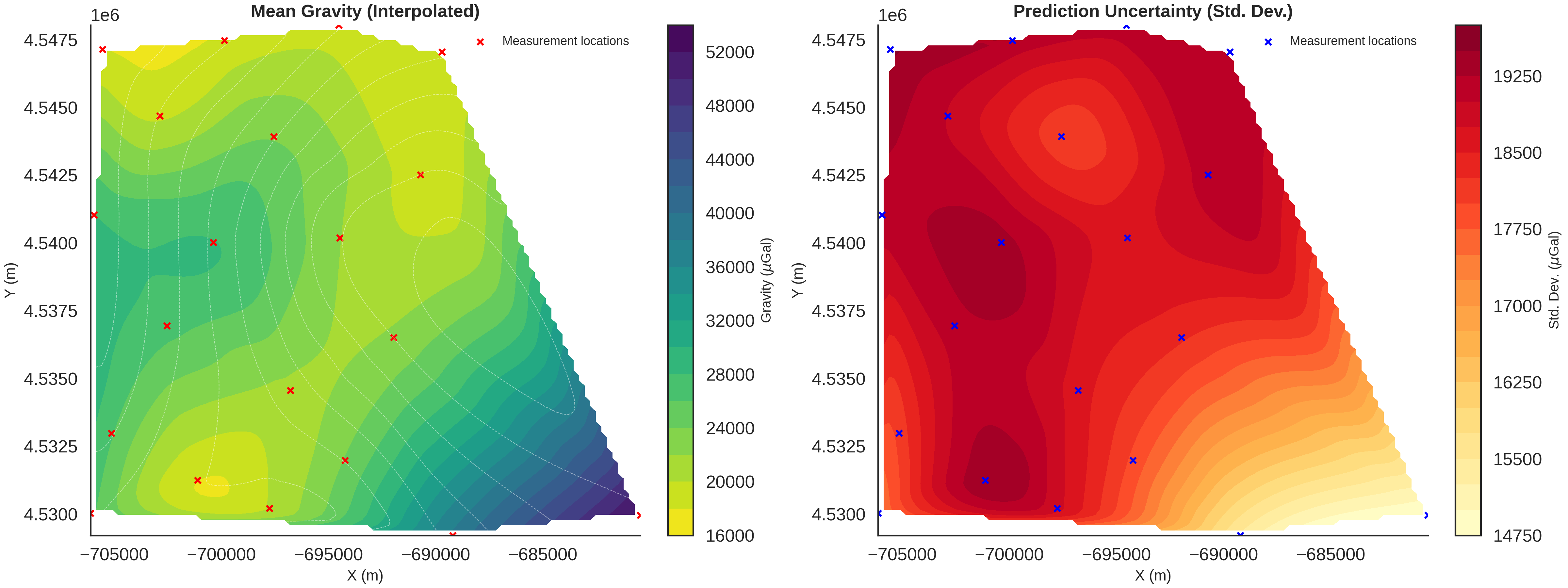
EXTRACTED NORMALIZED SAMPLES
============================================================
Number of samples: 100
Number of devices: 20
Normalization was applied DURING inference (not post-processing)
All samples use consistent normalization parameters from observed data
============================================================


============================================================
UNCERTAINTY SUMMARY STATISTICS
============================================================
Mean gravity:        24601.52 ± 8021.00 μGal
Mean uncertainty:    18425.53 μGal
Max uncertainty:     19551.38 μGal
Min uncertainty:     14735.75 μGal
Mean CV:             81.33%
RMSE:                9732.94 μGal
Correlation (R):     0.295
============================================================

if hasattr(data, 'posterior') and r'$\mu_{gravity}$' in data.prior:
    gravity_samples_norm, unit_label = generate_gravity_uncertainty_plots(
        gravity_samples_norm=data.posterior_predictive[r'$\mu_{gravity}$'].values[0, :],  # (n_samples, n_devices)
        observed_gravity_ugal=observed_gravity_ugal,
        xy_ravel=xy_ravel
    )

• 
• 
• 

============================================================
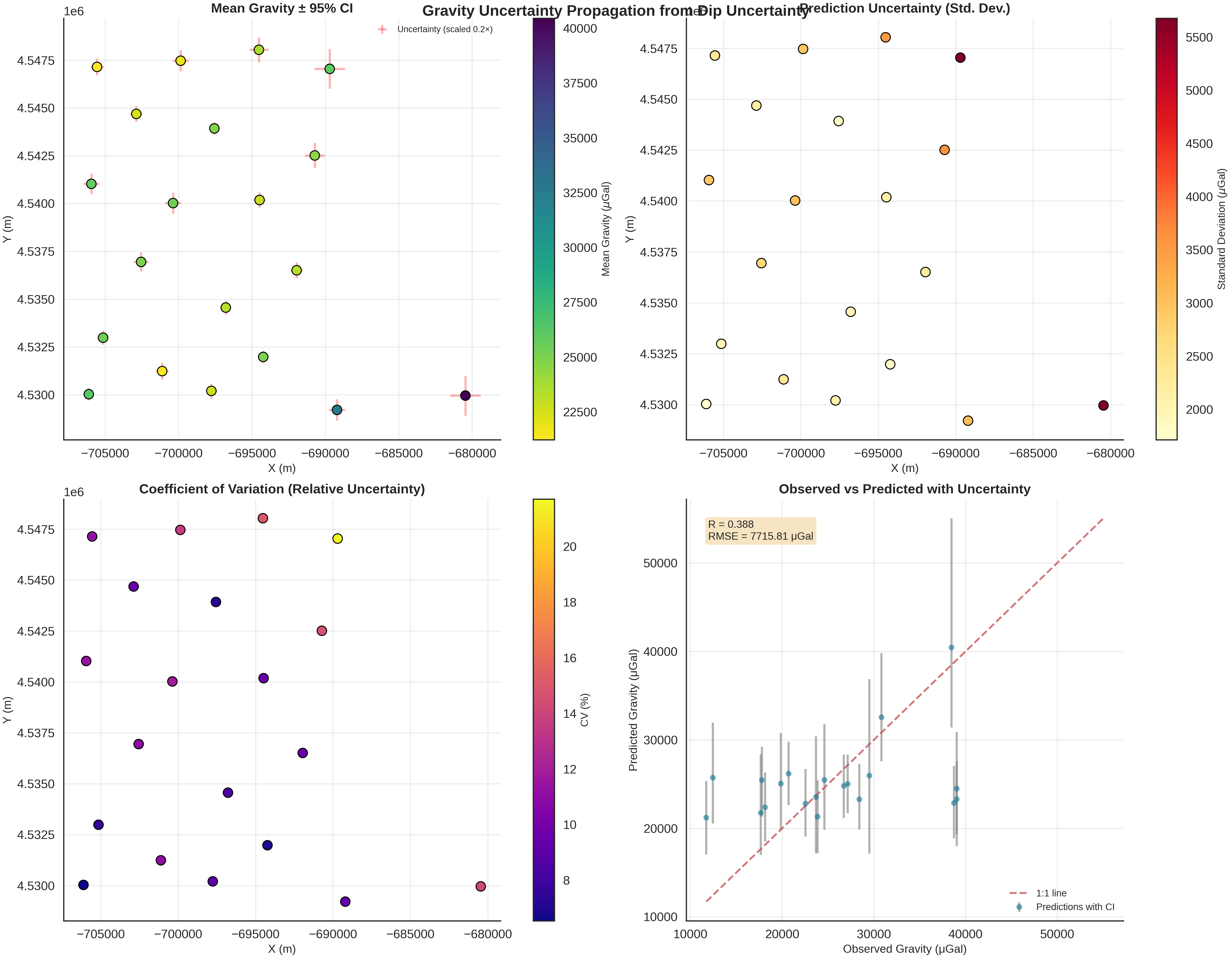
EXTRACTED NORMALIZED SAMPLES
============================================================
Number of samples: 200
Number of devices: 20
Normalization was applied DURING inference (not post-processing)
All samples use consistent normalization parameters from observed data
============================================================


============================================================
UNCERTAINTY SUMMARY STATISTICS
============================================================
Mean gravity:        25192.87 ± 4253.02 μGal
Mean uncertainty:    2785.16 μGal
Max uncertainty:     5678.72 μGal
Min uncertainty:     1713.74 μGal
Mean CV:             10.98%
RMSE:                7715.81 μGal
Correlation (R):     0.388
============================================================

Sigma Analysis: Outlier Detection

Hierarchical modeling allows us to identify stations with unusually high noise, which may indicate instrument problems, terrain correction errors, or localized geological complexity not captured by the model.

Stations where the inferred noise (sigma) is much higher than the global mean are candidates for being “problematic”.

if "sigma_stations" in data.posterior_predictive:
    posterior_sigmas = data.posterior_predictive["sigma_stations"].values
    station_noise_mean = posterior_sigmas.mean(axis=(0, 1))
    sigma_global_mean = station_noise_mean.mean()

    # Identify stations with noise > 2 standard deviations above mean
    problematic = np.where(station_noise_mean > 2 * sigma_global_mean)[0]
    print(f"\nPotential outlier stations identified: {problematic}")

    # Plot sigma distribution
    az.plot_density(
        data=[data, data.prior],
        var_names=["sigma_stations"],
        filter_vars="like",
        hdi_prob=0.9999,
        shade=.2,
        data_labels=["Posterior", "Prior"],
        colors=[default_red, default_blue],
    )
    plt.title("Per-Station Noise Distribution (Sigma)")
    plt.show()

Potential outlier stations identified: []

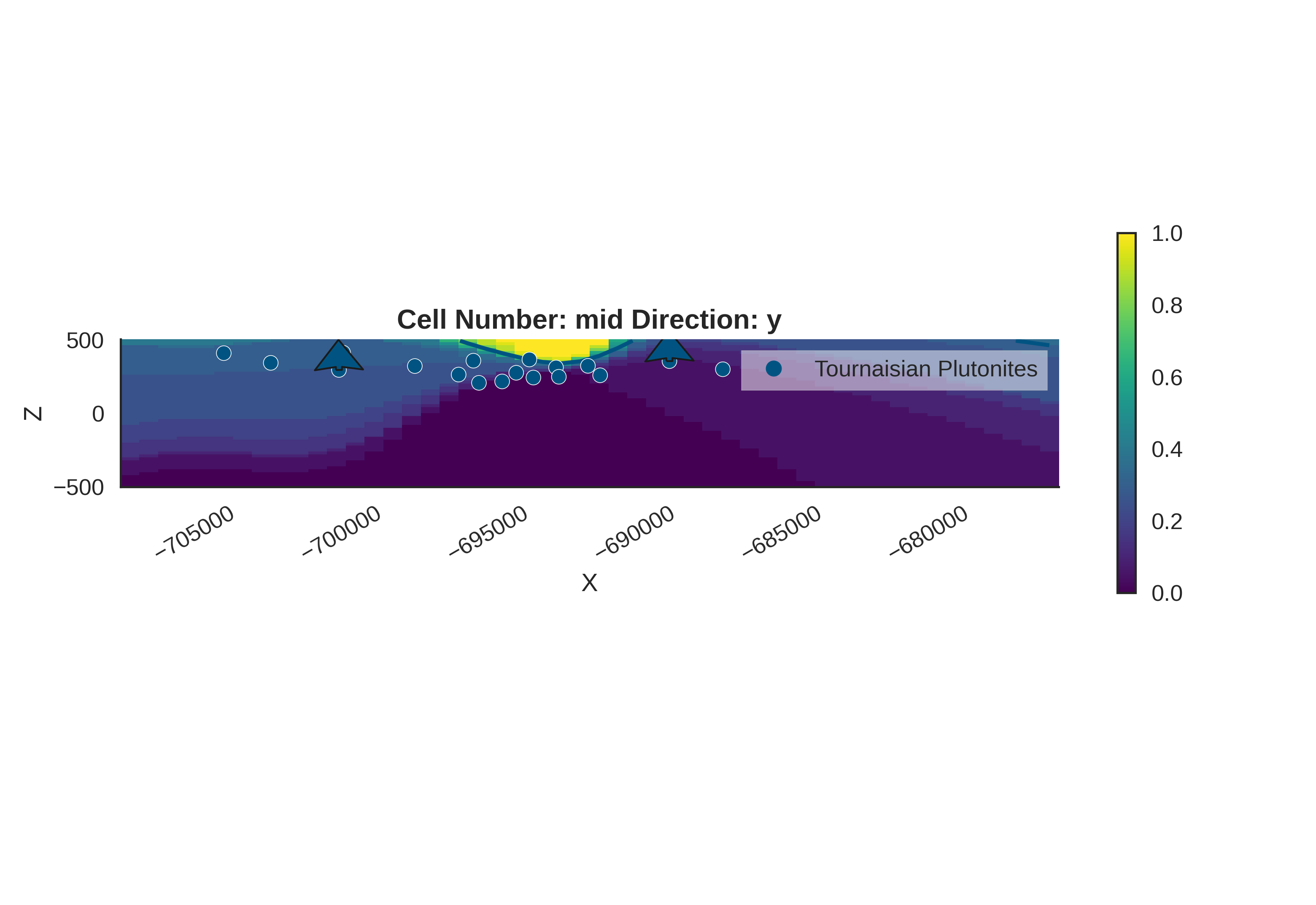
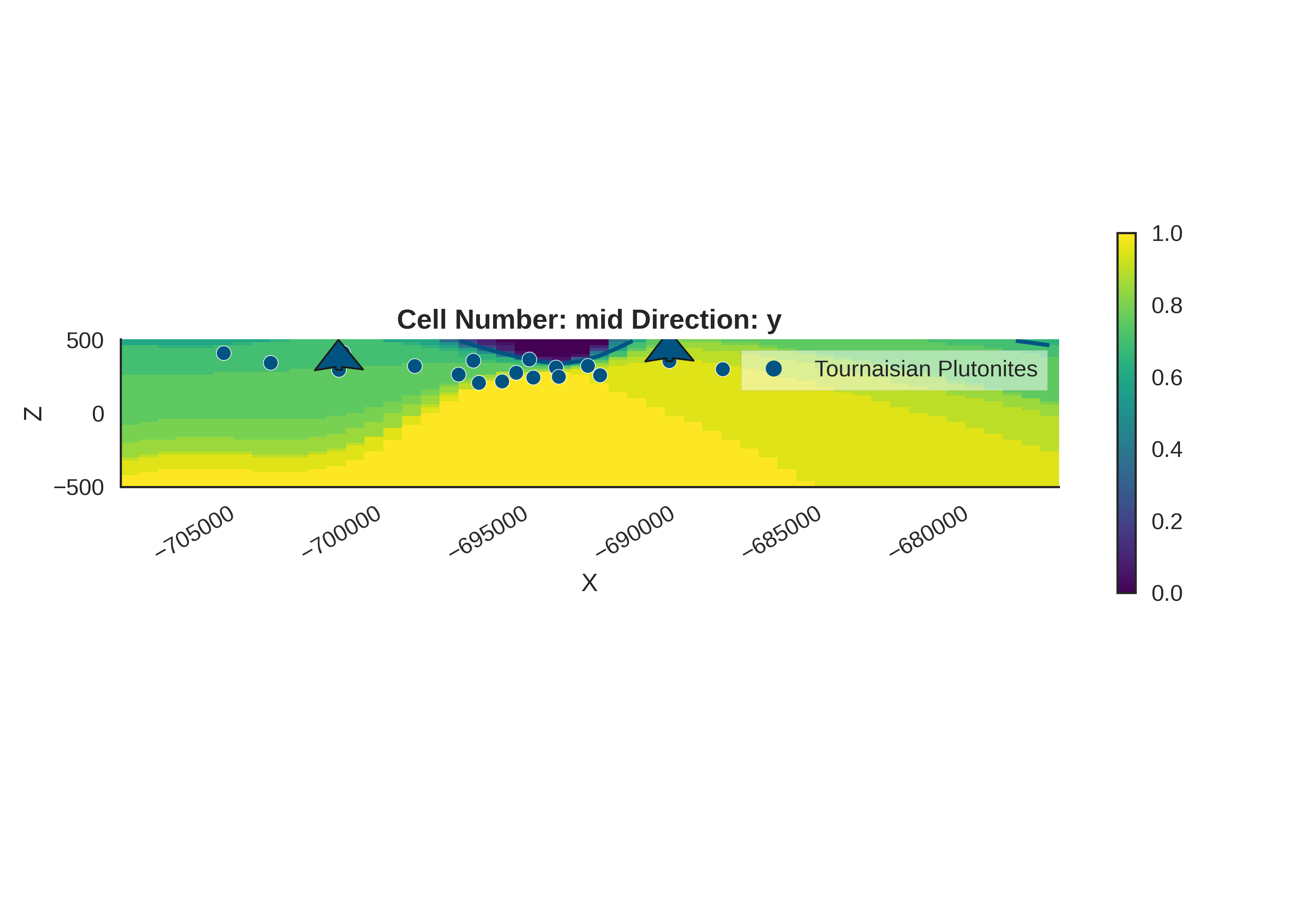
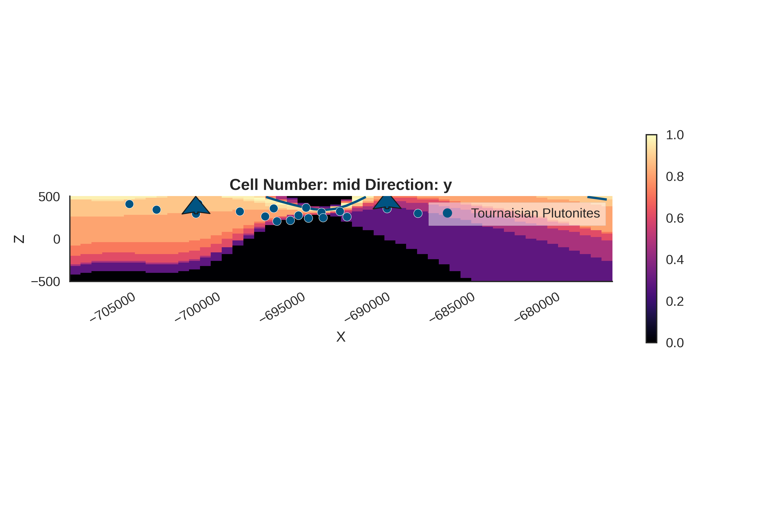
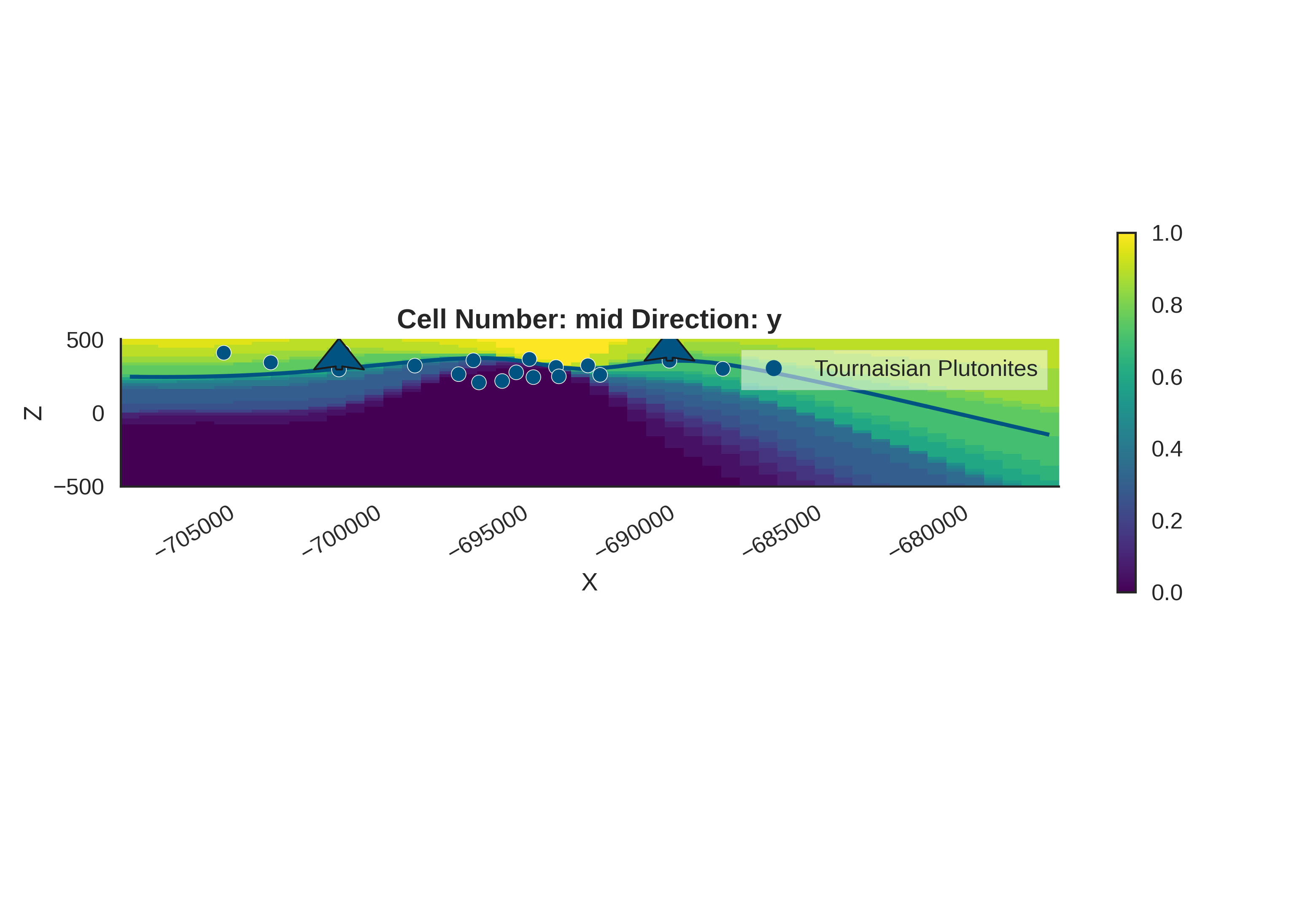
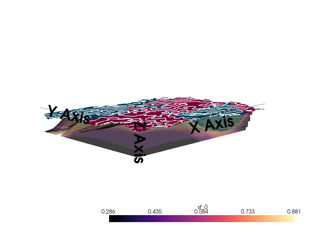
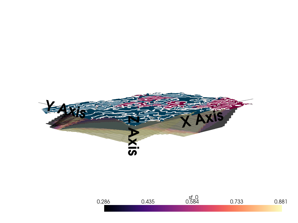
Probability Density Fields and Information Entropy

To visualize the spatial uncertainty of the geological structure, we compute probability density fields and information entropy.

• Probability Density Field: Shows the probability of each geological unit existing at any given location.

• Information Entropy: Quantifies the total uncertainty. High entropy means high uncertainty about which unit is present.

%% 3D Entropy Visualization

We can also visualize uncertainty in 3D by injecting the entropy field back into the GemPy solutions object.

Note: The 3D visualization is already handled inside probability_fields_for() by injecting the entropy field and calling gpv.plot_3d.

# Resetting the model
geo_model = gp.create_geomodel(
    project_name='gravity_inversion',
    extent=extent,
    refinement=refinement,
    resolution=resolution,
    importer_helper=gp.data.ImporterHelper(
        path_to_orientations=mod_or_path,
        path_to_surface_points=mod_pts_path,
    )
)

# Prior Probability Fields
print("\nComputing prior probability fields...")

topography_path = paths.get_topography_path()
probability_fields_for(
    geo_model=geo_model,
    inference_data=data.prior,
    topography_path=topography_path
)

# Posterior Probability Fields
if hasattr(data, 'posterior'):
    print("\nComputing posterior probability fields...")
    probability_fields_for(
        geo_model=geo_model,
        inference_data=data.posterior,
        topography_path=topography_path
    )

• 
• 
• 
• 
• 
• 

• 
• 

Computing prior probability fields...
Active grids: GridTypes.DENSE|NONE
Setting Backend To: AvailableBackends.PYTORCH
Using sequential processing for 1 surfaces
Setting Backend To: AvailableBackends.PYTORCH
Using sequential processing for 1 surfaces
Setting Backend To: AvailableBackends.PYTORCH
Using sequential processing for 1 surfaces
Setting Backend To: AvailableBackends.PYTORCH
Using sequential processing for 1 surfaces
Setting Backend To: AvailableBackends.PYTORCH
Using sequential processing for 1 surfaces
Setting Backend To: AvailableBackends.PYTORCH
Using sequential processing for 1 surfaces
Setting Backend To: AvailableBackends.PYTORCH
Using sequential processing for 1 surfaces
Setting Backend To: AvailableBackends.PYTORCH
Using sequential processing for 1 surfaces
Setting Backend To: AvailableBackends.PYTORCH
Using sequential processing for 1 surfaces
Setting Backend To: AvailableBackends.PYTORCH
Using sequential processing for 1 surfaces
Setting Backend To: AvailableBackends.PYTORCH
Using sequential processing for 1 surfaces
Setting Backend To: AvailableBackends.PYTORCH
Using sequential processing for 1 surfaces
Setting Backend To: AvailableBackends.PYTORCH
Using sequential processing for 1 surfaces
Setting Backend To: AvailableBackends.PYTORCH
Using sequential processing for 1 surfaces
Setting Backend To: AvailableBackends.PYTORCH
Using sequential processing for 1 surfaces
Setting Backend To: AvailableBackends.PYTORCH
Using sequential processing for 1 surfaces
Setting Backend To: AvailableBackends.PYTORCH
Using sequential processing for 1 surfaces
Setting Backend To: AvailableBackends.PYTORCH
Using sequential processing for 1 surfaces
Setting Backend To: AvailableBackends.PYTORCH
Using sequential processing for 1 surfaces
Setting Backend To: AvailableBackends.PYTORCH
Using sequential processing for 1 surfaces
Setting Backend To: AvailableBackends.PYTORCH
Using sequential processing for 1 surfaces
Active grids: GridTypes.DENSE|TOPOGRAPHY|NONE
Setting Backend To: AvailableBackends.PYTORCH
Using sequential processing for 1 surfaces
/home/leguark/PycharmProjects/gempy_viewer/gempy_viewer/modules/plot_3d/drawer_surfaces_3d.py:38: PyVistaDeprecationWarning:
../../../gempy_viewer/gempy_viewer/modules/plot_3d/drawer_surfaces_3d.py:38: Argument 'color' must be passed as a keyword argument to function 'BasePlotter.add_mesh'.
From version 0.50, passing this as a positional argument will result in a TypeError.
  gempy_vista.surface_actors[element.name] = gempy_vista.p.add_mesh(

Computing posterior probability fields...
Active grids: GridTypes.DENSE|NONE
Setting Backend To: AvailableBackends.PYTORCH
Using sequential processing for 1 surfaces
Setting Backend To: AvailableBackends.PYTORCH
Using sequential processing for 1 surfaces
Setting Backend To: AvailableBackends.PYTORCH
Using sequential processing for 1 surfaces
Setting Backend To: AvailableBackends.PYTORCH
Using sequential processing for 1 surfaces
Setting Backend To: AvailableBackends.PYTORCH
Using sequential processing for 1 surfaces
Setting Backend To: AvailableBackends.PYTORCH
Using sequential processing for 1 surfaces
Setting Backend To: AvailableBackends.PYTORCH
Using sequential processing for 1 surfaces
Setting Backend To: AvailableBackends.PYTORCH
Using sequential processing for 1 surfaces
Setting Backend To: AvailableBackends.PYTORCH
Using sequential processing for 1 surfaces
Setting Backend To: AvailableBackends.PYTORCH
Using sequential processing for 1 surfaces
Setting Backend To: AvailableBackends.PYTORCH
Using sequential processing for 1 surfaces
Setting Backend To: AvailableBackends.PYTORCH
Using sequential processing for 1 surfaces
Setting Backend To: AvailableBackends.PYTORCH
Using sequential processing for 1 surfaces
Setting Backend To: AvailableBackends.PYTORCH
Using sequential processing for 1 surfaces
Setting Backend To: AvailableBackends.PYTORCH
Using sequential processing for 1 surfaces
Setting Backend To: AvailableBackends.PYTORCH
Using sequential processing for 1 surfaces
Setting Backend To: AvailableBackends.PYTORCH
Using sequential processing for 1 surfaces
Setting Backend To: AvailableBackends.PYTORCH
Using sequential processing for 1 surfaces
Setting Backend To: AvailableBackends.PYTORCH
Using sequential processing for 1 surfaces
Setting Backend To: AvailableBackends.PYTORCH
Using sequential processing for 1 surfaces
Setting Backend To: AvailableBackends.PYTORCH
Using sequential processing for 1 surfaces
Active grids: GridTypes.DENSE|TOPOGRAPHY|NONE
Setting Backend To: AvailableBackends.PYTORCH
Using sequential processing for 1 surfaces
/home/leguark/PycharmProjects/gempy_viewer/gempy_viewer/modules/plot_3d/drawer_surfaces_3d.py:38: PyVistaDeprecationWarning:
../../../gempy_viewer/gempy_viewer/modules/plot_3d/drawer_surfaces_3d.py:38: Argument 'color' must be passed as a keyword argument to function 'BasePlotter.add_mesh'.
From version 0.50, passing this as a positional argument will result in a TypeError.
  gempy_vista.surface_actors[element.name] = gempy_vista.p.add_mesh(

Summary: The Complete Bayesian Gravity Inversion Workflow

Workflow Recap with Function Explanations

We’ve completed a full Bayesian gravity inversion. Here’s the complete pipeline with the role of each key function:

┌─────────────────────────────────────────────────────────────────┐
│ 1. PRIOR DEFINITION                                             │
│    Define prior distributions for parameters                    │
│    → model_priors = {dips: Normal(10, 10), density: Normal(...)}│
└─────────────────────────────────────────────────────────────────┘
                               ↓
┌─────────────────────────────────────────────────────────────────┐
│ 2. PROBABILISTIC MODEL CONSTRUCTION                             │
│    make_gempy_pyro_model_extended() orchestrates:               │
│    - Connects priors to GemPy via set_priors()                  │
│    - Defines forward model execution                            │
│    - Links predictions to data via likelihood_fn()              │
└─────────────────────────────────────────────────────────────────┘
                               ↓
┌─────────────────────────────────────────────────────────────────┐
│ 3. PRIOR PREDICTIVE CHECKS (gpp.run_predictive)                 │
│    Sample from prior to verify model adequacy:                  │
│    - gempy_viz() shows geological model uncertainty (KDE)       │
│    - plot_many_observed_vs_forward() checks if ANY prior        │
│      samples can explain observations                           │
└─────────────────────────────────────────────────────────────────┘
                               ↓
┌─────────────────────────────────────────────────────────────────┐
│ 4. MCMC INFERENCE (gpp.run_nuts_inference)                      │
│    For each iteration:                                          │
│    a) Sample θ from priors                                      │
│    b) set_priors(θ) → update GeoModel orientations & densities  │
│    c) Forward gravity computation                               │
│    d) Normalize & align to observations                         │
│    e) generate_multigravity_likelihood_hierarchical_per_station │
│       evaluates p(data|θ) with adaptive noise per station       │
│    f) NUTS uses ∇log p(data|θ) + ∇log p(θ) to propose next θ   │
└─────────────────────────────────────────────────────────────────┘
                               ↓
┌─────────────────────────────────────────────────────────────────┐
│ 5. POSTERIOR ANALYSIS                                           │
│    - plot_gravity_comparison() visualizes fit quality           │
│      * Shows observed, predicted, residuals, correlation        │
│    - az.plot_density() shows prior vs posterior distributions   │
│    - Posterior predictive checks validate model                 │
└─────────────────────────────────────────────────────────────────┘

Key Functions and Their Roles:

1. make_gempy_pyro_model_extended() - Central orchestrator connecting all components - Creates the probabilistic model structure - Enables automatic differentiation through entire workflow

2. set_priors() (passed as set_interp_input_fn) - Bridges Pyro samples → GemPy geological model - Converts sampled dip angles to gradient vectors - Updates densities in geophysics input

3. generate_multigravity_likelihood_hierarchical_per_station() - Creates robust likelihood with per-station noise inference - Automatically handles outliers via partial pooling - Returns function that computes p(observations|predictions)

4. plot_gravity_comparison() - 4-panel diagnostic showing observed vs predicted - Spatial residual patterns reveal model inadequacy - Correlation plot quantifies overall fit quality

5. plot_many_observed_vs_forward() - Shows if prior samples can explain observations - Crossing lines indicate parameter trade-offs - Essential for diagnosing prior mis-specification

6. gempy_viz() - Visualizes geological uncertainty via KDE - Overlays sample realizations on cross-sections - Compares prior vs posterior structural uncertainty

Key Insights from This Tutorial

1. Hierarchical modeling is powerful: By inferring per-station noise, we get automatic outlier detection without manual data cleaning.

2. Prior predictive checks are essential: Always verify that SOME combination of prior parameters can explain your data before running expensive MCMC.

3. Residual patterns tell a story:

   • Random residuals → good model fit

   • Spatial patterns → missing geological complexity

   • Systematic bias → wrong physics or normalization

4. Geological inversions are regression problems: Just as y = θ₁x + θ₂ in linear regression, here y = f(θ) where f is complex geological simulation. Same statistical principles apply!

5. Multiple data views matter: Use gempy_viz, plot_gravity_comparison, and plot_many_observed_vs_forward together for comprehensive understanding.

Next Steps for Production Inversions

To enhance this workflow for real-world applications:

1. Run multiple chains (num_chains=4): Diagnose convergence with R-hat statistic

2. Increase samples: 200 is minimal; use 1000+ for publication-quality results

3. More parameters: Invert for layer thicknesses, additional orientations, spatially-varying densities, fault locations

4. Joint inversion: Combine gravity with magnetics, seismic, or MT data for tighter constraints

5. Model comparison: Use LOO-CV or WAIC to compare alternative geological hypotheses (e.g., 2-layer vs 3-layer models)

6. Sensitivity analysis: Systematically vary priors to assess robustness

7. Forward uncertainty propagation: Use posterior samples to quantify uncertainty in derived quantities (ore tonnage, depth to target, etc.)

Diagnostic Checks Available (not all shown in this tutorial):

• Convergence: R-hat < 1.01, ESS > 400 per chain

• Trace plots: Check for mixing and stationarity

• Divergences: Should be < 1% of samples (indicates problematic geometry)

• Energy plots: Diagnose sampler efficiency

• Posterior predictive p-values: Assess model adequacy

• Leave-one-out cross-validation: Predict held-out stations

Congratulations! You now understand how to: - Build complex geological forward models - Define hierarchical Bayesian likelihoods - Integrate geophysical data with geological priors - Diagnose and visualize inference results - Extend this framework to your own problems

# sphinx_gallery_thumbnail_number = 7