Simple Geological Model - Tharsis Region

This example creates a simple 3D geological model of the Tharsis region using GemPy.

Overview

The Tharsis mining district in southwestern Spain is part of the Iberian Pyrite Belt (IPB), one of the world’s most important volcanogenic massive sulfide (VMS) provinces. This example demonstrates the fundamental workflow for creating a 3D geological model from structural data.

Geological Context

The Tharsis deposit consists primarily of Tournaisian-age plutonites that intrude into older Devonian basement rocks. The intrusion created significant hydrothermal alteration and mineralization, making it a target for geophysical exploration methods.

Technical Details

This model uses:

• Octree refinement (level 5): Adaptive mesh refinement that concentrates computational effort near geological interfaces while maintaining efficiency in homogeneous regions

• Real structural data: Surface contact points and orientation measurements from field mapping

• Topographic integration: High-resolution DEM to accurately represent surface geology

Note

The coordinate system uses UTM Zone 29N projection (EPSG:32629) with elevations in meters above sea level.

Import Libraries

We use GemPy for 3D implicit geological modeling. GemPy uses a universal co-kriging interpolation approach to construct continuous 3D geological surfaces from sparse data points.

Universal Co-Kriging

GemPy’s core interpolation engine is based on Universal Co-Kriging, a geostatistical method that combines multiple types of information into a single consistent 3D model.

\[Z(x) = \sum_{i=1}^n \lambda_i Z(x_i) + \sum_{j=1}^m \beta_j f_j(x)\]

Where:

• \(Z(x)\) is the value of the potential field at location \(x\)

• \(\sum \lambda_i Z(x_i)\) represents the kriging part (honoring point data)

• \(\sum \beta_j f_j(x)\) represents the universal part (honoring orientations/gradients)

This approach ensures that the resulting surfaces are both continuous and honor all structural constraints simultaneously.

NumPy provides numerical computing capabilities for array operations.

import numpy as np
import gempy as gp

# Set random seed for reproducibility
np.random.seed(1234)

Setting Backend To: AvailableBackends.PYTORCH

Import paths configuration

from mineye.config import paths

Define Model Extent and Resolution

The model covers the Tharsis mining district in UTM coordinates (Zone 29N).

Model Extent: The bounding box defines the 3D volume for interpolation:

• X range: 33.96 km (East-West direction)

• Y range: 25.12 km (North-South direction)

• Z range: 1.005 km (from -500m to +505m elevation)

The vertical extent captures both subsurface structures (down to 500m below sea level) and topography (up to 505m above sea level).

min_x = -707_521  # * Cropping the corrupted area of the geotiff
max_x = -675558
min_y = 4526832
max_y = 4551949
max_z = 505
model_depth = -500
extent = [min_x, max_x, min_y, max_y, model_depth, max_z]

# **Model resolution**: use octree with refinement level 5
#
# Octree refinement adaptively subdivides the model space:
#
# * Level 5 creates up to 2^5 = 32 subdivisions per dimension
# * Finer resolution near geological contacts
# * Coarser resolution in homogeneous regions
# * Significantly more efficient than regular grids for complex geometries
resolution = None  # Using octrees instead of regular grid
refinement = 5

Get Data Paths

Load paths to structural data

Structural geological data consists of two types:

1. Surface points: 3D coordinates (X, Y, Z) marking where geological contacts were observed, typically from field mapping, drill holes, or cross-sections

2. Orientations: The 3D orientation (dip, azimuth) of geological surfaces at specific locations, providing information about how surfaces trend through space

These data constrain the implicit interpolation algorithm to construct geologically plausible 3D surfaces.

mod_or_path = paths.get_orientations_path()
mod_pts_path = paths.get_points_path()

print(f"Orientations: {mod_or_path}")
print(f"Points: {mod_pts_path}")

Orientations: /home/leguark/PycharmProjects/Mineye-Terranigma/examples/Data/Model_Input_Data/Simple-Models/orientations_mod.csv
Points: /home/leguark/PycharmProjects/Mineye-Terranigma/examples/Data/Model_Input_Data/Simple-Models/points_mod.csv

Create GemPy Geological Model

Build the model structure with imported structural data

GemPy’s implicit modeling approach:

• Uses a universal co-kriging interpolator to construct smooth 3D scalar fields

• Each geological surface is represented as an isosurface of a scalar field

• The gradient of the scalar field (orientation data) and the isovalue (surface points) constrain the interpolation

• The result is a continuous 3D model that honors all input data

The ImporterHelper automatically reads and formats CSV files containing the structural data.

simple_geo_model = gp.create_geomodel(
    project_name='simple_model',
    extent=extent,
    refinement=refinement,
    resolution=resolution,
    importer_helper=gp.data.ImporterHelper(
        path_to_orientations=mod_or_path,
        path_to_surface_points=mod_pts_path,
    )
)

Map Geological Units

Define the stratigraphic stack

Stratigraphic series organize geological formations into age-related groups. In GemPy, each series can contain multiple surfaces (formations) that are interpolated together using the same scalar field.

For this simple model, we have a single series containing the Tournaisian Plutonites. This intrusive body represents the youngest geological unit in the model, with all other rocks implicitly treated as the “basement” by GemPy.

In more complex models, you would define multiple series representing different geological events (e.g., sedimentation, folding, faulting, intrusion).

gp.map_stack_to_surfaces(
    gempy_model=simple_geo_model,
    mapping_object={
            "Tournaisian_Plutonites": ["Tournaisian Plutonites"],
    }
)

Structural Groups:	StructuralGroup: Name: Tournaisian_Plutonites Structural Relation: StackRelationType.ERODE Elements: StructuralElement: Name: Tournaisian Plutonites
Fault Relations:	Tournaisia... Tournaisian_Plutonites
	True False

Compute Model with Topography

Add topographic surface from DEM and compute the model

Digital Elevation Models (DEMs) provide high-resolution surface topography that significantly improves the accuracy of near-surface geological modeling.

Importance of topography in geological modeling:

• Defines the true upper boundary of the model (not just a flat plane)

• Critical for geophysical modeling (gravity, magnetics) where topography affects measurements

• Enables accurate calculation of true thickness of geological units

• Important for resource estimation and mine planning

The DEM is loaded from a raster file and resampled to match the model grid. GemPy automatically clips the geological model at the topographic surface, ensuring that geological units only exist below ground.

topography_path = paths.get_topography_path()
gp.set_topography_from_file(
    grid=simple_geo_model.grid,
    filepath=topography_path,
    crop_to_extent=[
            simple_geo_model.grid.extent[0],
            simple_geo_model.grid.extent[2],
            simple_geo_model.grid.extent[1],
            simple_geo_model.grid.extent[3]
    ]
)

# Compute the model with topography
gp.compute_model(simple_geo_model)

Active grids: GridTypes.OCTREE|TOPOGRAPHY|NONE
Setting Backend To: AvailableBackends.PYTORCH
Using sequential processing for 1 surfaces
/home/leguark/.venv/2025/lib/python3.13/site-packages/torch/utils/_device.py:103: UserWarning: Using torch.cross without specifying the dim arg is deprecated.
Please either pass the dim explicitly or simply use torch.linalg.cross.
The default value of dim will change to agree with that of linalg.cross in a future release. (Triggered internally at /pytorch/aten/src/ATen/native/Cross.cpp:63.)
  return func(*args, **kwargs)

Solutions: 5 Octree Levels, 1 DualContouringMeshes

Visualize the Model

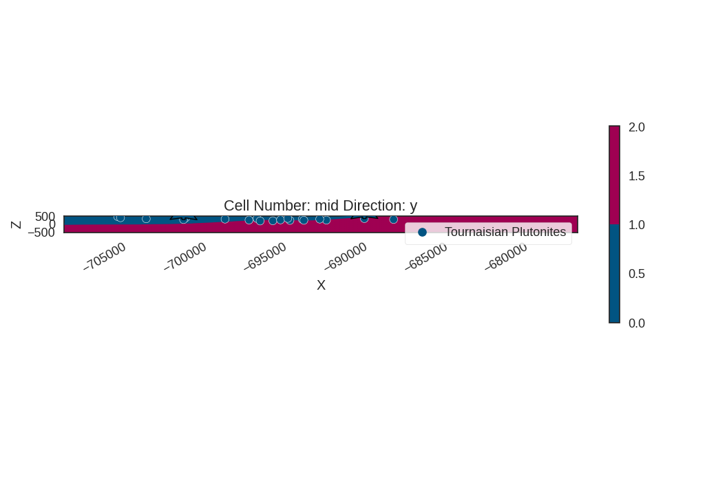
2D Cross-Sections

Before diving into 3D, it’s often helpful to inspect 2D cross-sections. This allows for a clear view of the internal structural relationships and the behavior of the interpolator along specific planes.

We’ll plot a cross-section along the Y-axis (North-South) at the center of the model.

import gempy_viewer as gpv

gpv.plot_2d(simple_geo_model, direction='y', cell_number='mid', show_data=True)

<gempy_viewer.modules.plot_2d.visualization_2d.Plot2D object at 0x7f2db0ed9940>

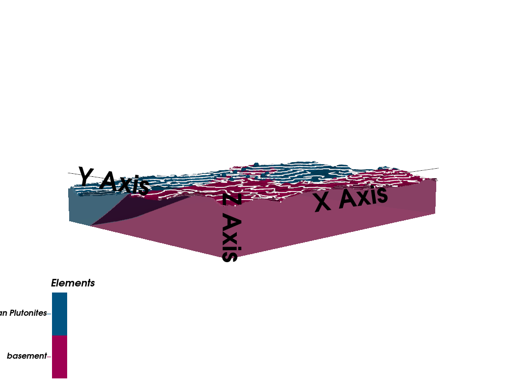
3D Visualization

Create 3D visualization of the geological model

GemPy Viewer provides interactive 3D visualization capabilities using PyVista.

Visualization features:

• 3D lithology blocks: Colored volumes representing different geological units

• Topographic surface: The DEM draped over the model

• Input data: Surface points and orientation measurements shown in 3D space

• Vertical exaggeration (ve=5): Stretches the Z-axis by a factor of 5 to enhance the visibility of subtle geological features

The visualization is fully interactive, allowing rotation, zooming, and inspection of the geological model from any angle.

import gempy_viewer as gpv

gpv.plot_3d(simple_geo_model, ve=5, image=False,
            kwargs_pyvista_bounds={
                    'show_xlabels': False,
                    'show_ylabels': False,
                    'show_zlabels': False
            }
            )

/home/leguark/PycharmProjects/gempy_viewer/gempy_viewer/modules/plot_3d/drawer_surfaces_3d.py:38: PyVistaDeprecationWarning:
../../../gempy_viewer/gempy_viewer/modules/plot_3d/drawer_surfaces_3d.py:38: Argument 'color' must be passed as a keyword argument to function 'BasePlotter.add_mesh'.
From version 0.50, passing this as a positional argument will result in a TypeError.
  gempy_vista.surface_actors[element.name] = gempy_vista.p.add_mesh(

<gempy_viewer.modules.plot_3d.vista.GemPyToVista object at 0x7f2db1026ba0>

Summary and Next Steps

In this example, we demonstrated the complete workflow for creating a simple 3D geological model using GemPy:

1. ✓ Defined the model extent and resolution

2. ✓ Imported structural geological data (surface points and orientations)

3. ✓ Created a GemPy geomodel with stratigraphic organization

4. ✓ Computed the 3D geological model using implicit interpolation

5. ✓ Integrated high-resolution topography from a DEM

6. ✓ Visualized the resulting 3D model

Key Takeaways:

• GemPy uses implicit modeling to create continuous 3D geological surfaces from sparse data

• Octree refinement provides efficient adaptive resolution

• Topography integration is crucial for accurate geological modeling

• The resulting model can be used for further analysis (geophysics, resource estimation, etc.)

Next Steps:

• Example 02: Forward gravity modeling using this geological model

• Example 03: Bayesian segmentation for lithological mapping

• Probabilistic examples: Uncertainty quantification and joint inversion

See also

• GemPy Documentation

• PyVista for 3D Visualization

sphinx_gallery_thumbnail_number = 2